Retraining Cellpose on Custom Data

Download this Notebook Open in Colab

# /// script
# requires-python = ">=3.12"
# dependencies = [
#     "matplotlib",
#     "cellpose",
# ]
# ///

Overview

Website | GitHub | Paper | Cellpose Documentation | Cellpose API

In this section, we will walk through how to retrain Cellpose on your own data. This is useful when the default models don’t perform well on your specific cell type, staining method, or imaging modality.

Retraining allows Cellpose to learn directly from your examples, leading to better segmentation accuracy and more relevant masks for your experiments.

To go through the training process, you need pairs of raw microscopy images and their corresponding label masks. The raw images are what you want to segment, and the label masks are the ground truth segmentations that the model will learn from.

The images we will use for this section can be downloaded from the Cellpose Training Dataset.

⚠️ Tip: Cellpose runs significantly faster on a GPU. It supports both NVIDIA GPUs (CUDA) and Apple Silicon (MPS). If you don't have either, we recommend running this notebook on Google Colab for faster performance.

NVIDIA GPU (CUDA - Windows/Linux)

In order to use Cellpose in this notebook with an NVIDIA GPU:

1. you need to have the NVIDIA drivers installed on your system.

2. you can run nvidia-smi in the terminal to check your CUDA version (shown in the top-right of the output, e.g. CUDA Version: 13.0.0).

3. update the # /// script block at the top of this notebook to install the appropriate version of PyTorch with CUDA support (replace cu130 with your CUDA version):

    # /// script
    # requires-python = ">=3.12"
    # dependencies = [
    #     "matplotlib",
    #     "cellpose",
    #     "torch",
    #     "torchvision",
    # ]
    #
    # [tool.uv.sources]
    # torch = { index = "pytorch-cu130" }
    # torchvision = { index = "pytorch-cu130" }
    #
    # [[tool.uv.index]]
    # name = "pytorch-cu130"
    # url = "https://download.pytorch.org/whl/cu130"
    # explicit = true
    # ///

4. re-run the notebook using uvx juv run.

How to Retrain Cellpose

In this tutorial we will cover the retraining process using the code-based approach.

However, the retraining process can also be performed interactively using the Cellpose GUI. To launch the Cellpose GUI, you can follow the instruction in the Introduction to Cellpose section. For more information you can also check the Cellpose documentation.

Data

For this tutorial, we will use the sample dataset provided by Cellpose, which includes both training and test images pairs. You can download the dataset here: Cellpose Training Dataset.

🚧 Note: We will use only the sample dataset provided by Cellpose to demonstrate the retraining pipeline. If you want to retrain Cellpose on your own data, you will probably need more image pairs for training and for testing, as well as some validation data.

Creating Label Masks

As mentioned above, the dataset we will use already includes label masks, but if you want to retrain Cellpose on your own data, you will need to create these masks yourself.

There are different tools available. One example is the Cellpose GUI itself, which lets you modify and save updated labels in a user-friendly way. You can see the Cellpose documentation for more details on how to create and edit label masks.

Another option is to use annotation tools like napari. If using uv, you can simply start napari by running in your terminal:

uvx "napari[all]"

The napari GUI will open and you can load your raw images and create or modify and then save the corresponding label masks using the annotation tools available.

💡 Tip: After adding your labelled masks into napari, to convert them into a Labels layer, simply right-click on it and select Convert to Labels.

Retraining Pipeline

The retraining pipeline consists of the following steps:

1. Data Preparation: Organize your raw images and label masks into a format that Cellpose can use for training.

2. Model Configuration: Set up the training parameters, such as the number of epochs, learning rate, and batch size.

3. Run the standard model on test data [optional]: Before training, in this tutorial we will run the standard Cellpose model on the test data to see how it performs before retraining.

4. Train the Model: Use the prepared data to train a new Cellpose model.

5. Evaluate the Model: After training, evaluate the performance of the new model on the test data and compare it to the performance of the standard model.

Retraining for 3D Data

train.train_seg always trains a 2D network, even for 3D segmentation. When you run inference with do_3D=True, Cellpose applies this 2D network to the XY, XZ and YZ slices of the volume and combines the resulting flows (see the 3D segmentation documentation).

This means that if your data is 3D and the default/pretrained model doesn’t perform well in do_3D mode, your training set should not consist only of XY slices. To get a model that segments well in all three orientations, you should provide labelled 2D image/mask pairs sampled from all three orthogonal planes of your annotated volumes:

• XY slices (the standard top-down view)

• XZ slices (a vertical “side” view)

• YZ slices (the other vertical “side” view)

Mixing slices from the three planes into your train (and test) folders teaches the network what objects look like from every orientation, so that the flows it predicts on XZ/YZ slices during 3D inference are as accurate as the ones it predicts on XY slices.

Generating multi-plane training crops

Cellpose provides a helper script, make_train.py, that extracts random XY, XZ and YZ crops from a 3D image (and its label volume, if available) and saves them as 2D .tif files ready to be labelled (or corrected) in the Cellpose GUI. Note that this script needs a local display, so it can’t be run on Colab; run it locally instead.

python -m cellpose.gui.make_train --dir /path/to/3d/data --anisotropy 5

Use --anisotropy (the ratio of the Z pixel size to the XY pixel size, the same value you would pass to model.eval(..., anisotropy=...)) so that the XZ/YZ crops are rescaled to look isotropic, matching the appearance of the XY crops.

Once you have a folder of labelled 2D image/mask pairs covering all three planes, you can use them with train.train_seg exactly as shown below: no extra 3D-specific parameters are needed, since the network itself only ever sees 2D slices.

Import Libraries

from pathlib import Path

import matplotlib.pyplot as plt
from cellpose import core, io, metrics, models, train

Setup

io.logger_setup()  # to get printing of progress

use_gpu = core.use_gpu()
print("GPU available:", use_gpu)

Data Handling

Cellpose expects images and their corresponding masks to live in the same folder. The file names must share the same prefix and only differ by the suffix. For example, if the raw image is named img_0.tif, the corresponding mask should be named img_0_seg.tif (_seg here is just an example, you can use any suffix you like).

You’ll also need to split your data into a train and a test folder. The model learns from the training set and is evaluated on the test set (images it has never seen during training).

cellpose_data/
├── train/
│   ├── img_0.tif
│   ├── img_0_seg.tif
│   ├── img_1.tif
│   ├── img_1_seg.tif
│   └── ...
└── test/
    ├── img_8.tif
    ├── img_8_seg.tif
    ├── img_9.tif
    ├── img_9_seg.tif
    └── ...

After organizing your data, the first step is to define the train and test directories, then load the data with io.load_train_test_data, passing the mask (and image if needed) suffixes so Cellpose can pair them correctly.

ROOT_FOLDER_PATH = Path("data/05_segmentation_cellpose_training")

train_dir = ROOT_FOLDER_PATH / "train"
test_dir = ROOT_FOLDER_PATH / "test"

# add name filters to select only images and masks from the folders
# `mask_filter` identifies mask files by their suffix
# (e.g. "_seg" for files like "img_000_seg". If not .tif, add also the extension).
mask_filter = "_seg"

# if necessary, you can also specify an `image_filter` to select images with a specific
# suffix (e.g. "_img" for files like "img_000_raw.tif". If not .tif, add also the extension).
# image_filter = "_raw"

# Load training and test data
output = io.load_train_test_data(
    str(train_dir),
    str(test_dir),
    mask_filter=mask_filter,
    # image_filter=image_filter
)

# assign the output to the appropriate variables
train_data, train_labels, _, test_data, test_labels, _ = output

Initialize the Model

To initialize Cellpose model we can use the models.CellposeModel() class.

There are other parameters we can set when initializing the model, here we will only use pretrained_model to specify which pretrained model to use and gpu to specify whether to use GPU (if available) for faster inference.

Currently, the available pretrained models are:

• cpsam: this is the original CellposeSAM model released in April 2025 using the SAM-ViTL backbone (default model)

• cpsam_v2: this is the CellposeSAM model released in June 2026 using the SAM-ViTL backbone, it includes a fix in the training for low contrast regions

• cpdino: this is the CellposeDINO model released in June 2026 using the DINOv3-ViTL backbone

• cpdino-vitb: this is the CellposeDINO model released in June 2026 using the DINOv3-ViTB backbone (smaller model)

Note: Only the default cpsam model is downloaded automatically the first time you run this notebook (this may take a while). The other models (cpsam_v2, cpdino, cpdino-vitb) must be downloaded manually, see below.

Downloading the Other Pretrained Models

These models are hosted on the Cellpose-SAM Hugging Face repository. We need to download the model weights and place them in the ~/.cellpose/models directory (the MODEL_DIR variable from the cellpose.models module).

from cellpose.models import MODEL_DIR
from cellpose.utils import download_url_to_file

model_name = "cpsam_v2"  # or "cpdino" / "cpdino-vitb"

MODEL_DIR.mkdir(parents=True, exist_ok=True)
model_path = MODEL_DIR / model_name
if not model_path.exists():
    url = f"https://huggingface.co/mouseland/cellpose-sam/resolve/main/{model_name}"
    download_url_to_file(url, str(model_path))

model_path = str(MODEL_DIR / "cpsam_v2")  # or "cpdino" / "cpdino-vitb" or "cpsam"
model = models.CellposeModel(pretrained_model=model_path, gpu=use_gpu)

How does a model perform on the test data?

Before training a new model, let’s see how the pre-trained Cellpose model we chose performs on the test data.

# run model on test images
masks, _, _ = model.eval(test_data, batch_size=8)

Now we’ll quantify how well the standard model segments the test images by comparing the predicted masks to the ground truth labels using metrics.average_precision.

For each test image, every predicted mask is matched to a ground truth mask based on their Intersection over Union (IoU): the overlap area divided by the union area of the two masks.

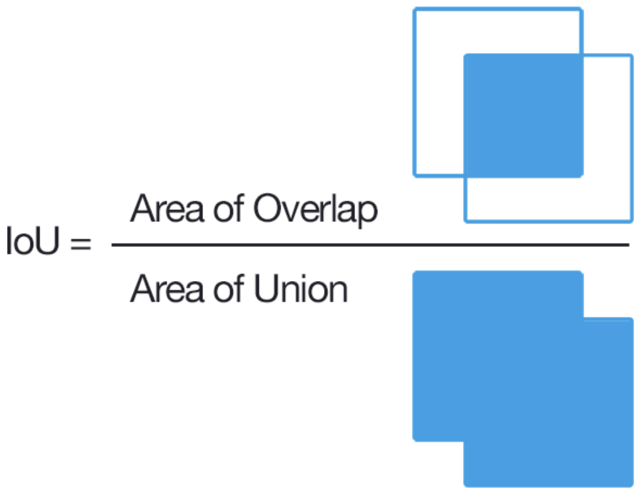
A predicted mask counts as a true positive (TP) if its IoU with a ground truth mask is above a given threshold; otherwise it is a false positive (FP), and any unmatched ground truth mask is a false negative (FN). The average precision (AP) is then computed as:

\[ AP = \frac{TP}{TP + FP + FN} \]

By default, metrics.average_precision computes this at IoU thresholds of 0.5, 0.75, and 0.9. A higher threshold requires a tighter overlap between predicted and ground truth masks, so AP typically decreases as the threshold increases. Comparing these values before and after retraining gives us a quantitative measure of how much the model improves on our data.

# check performance using ground truth labels
# average_precision returns AP at IoU thresholds [0.5, 0.75, 0.9] by default
values = metrics.average_precision(test_labels, masks)
average_precision, _, _, _ = values

print(f"average precision at iou threshold 0.5  = {average_precision[:, 0].mean():.3f}")
print(f"average precision at iou threshold 0.75 = {average_precision[:, 1].mean():.3f}")
print(f"average precision at iou threshold 0.9  = {average_precision[:, 2].mean():.3f}")

Let’s now visualize the results for the test images.

n = 0  # test image index to visualize
cyto_ch = 1  # channel index for cytoplasm (0=nucleus, 1=cytoplasm in this dataset)
raw_data = test_data[n][cyto_ch]  # selecting which test data ans which channel
pred_mask = masks[n]  # selecting the predicted mask for the same test image
gt_mask = test_labels[n]  # selecting the ground truth mask for the same test image

plt.figure(figsize=(10, 5))
plt.subplot(1, 3, 1)

plt.imshow(raw_data, cmap="gray")
plt.title(f"Test Image {n}")
plt.axis("off")

plt.subplot(1, 3, 2)
plt.imshow(pred_mask, cmap="nipy_spectral")
plt.title(f"Predicted Mask {n}")
plt.axis("off")

plt.subplot(1, 3, 3)
plt.imshow(gt_mask, cmap="nipy_spectral")
plt.title(f"GT Mask {n}")
plt.axis("off")

plt.tight_layout()
plt.show()

Train New Model

Now we’re ready to retrain Cellpose using the train_seg method from the train module.

Here we will change few training parameters but you can find the full parameters description for the train.train_seg method in the dropdown below or in the Cellpose API documentation

Cellpose train.train_seg() Parameters

Input Data

Parameter	Default	What it does
train_data	None	List of numpy arrays (2D or 3D images). Mutually exclusive with train_files, use one or the other.
train_labels	None	List of integer label arrays matching train_data. 0 = background, 1, 2, ... = individual masks.
train_files	None	File paths to training images. Used instead of train_data when loading from disk. Use together with load_files=True (the default), this is the standard path when working from disk.
train_labels_files	None	File paths to the corresponding label files.
test_data / test_labels	None	Same as above but for validation. Used only to report test loss, does not affect gradient updates.
test_files / test_labels_files	None	Same as above, file-based version.
load_files	True	If True, loads images/labels from the *_files paths at the start of training. Set to False if you’ve already loaded them into arrays and don’t want redundant I/O.
channel_axis	None	Which axis in the arrays is the channel axis. None = infer automatically.

Sampling & Epoch Control

Parameter	Default	What it does
train_probs	None	Per-image sampling probability for each epoch. If None, all images get equal weight (1/n). The right lever if you want to hard-mine difficult images or balance an uneven dataset. Must sum to 1 after normalization.
test_probs	None	Same for test images.
nimg_per_epoch	None	How many images (with random augmentation each time) Cellpose samples per epoch, doing one gradient update per image. If None, defaults to len(train_data). For a large dataset (50/100+ images), leave as None, one pass per epoch is already enough gradient steps. For a small dataset (5-10 images), set it higher than your dataset size (e.g. 50 or 100 for 5 images): each image gets sampled multiple times per epoch with different random augmentations (crop, rotation, flip, scale), and more updates/epoch help the linear LR warmup over the first 10 epochs actually move the weights.
nimg_test_per_epoch	None	Same as nimg_per_epoch but for test loss reporting only, it does not affect training. For a small test set (2-5 images), leave as None (uses all) for a stable loss estimate, subsampling a tiny test set gives noisy numbers. For a large test set (100+ images), set it lower (e.g. 20) to speed up per-epoch evaluation at the cost of noisier test loss curves.
min_train_masks	5	Images with fewer than this many mask instances are silently dropped before training starts, guarding against nearly-empty label images corrupting training. If your dataset is small, check how many images actually survive this filter.

Optimizer

Parameter	Default	What it does
learning_rate	1e-5	learning rate (LR) for the AdamW algorithm used by Cellpose. Controls how large each weight update is. Too high → the model overshoots and training becomes unstable (loss oscillates). Too low → the model learns very slowly or gets stuck. For fine-tuning a pre-trained model like Cellpose, a small value is preferred to avoid erasing what the model already knows (e.g. 1e-5 or 0.00001). Note that learning_rate is also ramped up linearly from 0 to its target value over the first 10 epochs (regardless of n_epochs), so with very few epochs the target learning rate may never be reached.
weight_decay	0.1	AdamW algorithm weight decay (L2 regularization). 0.1 is the modern default from the AdamW paper.
SGD	False	Deprecated as of v4.0.1. AdamW is always used regardless of this value.
n_epochs	100	one epoch = one full pass through all training images. More epochs give the model more time to learn, but too many can lead to overfitting: the model memorizes the training data and performs worse on new images. Watch the test loss, if it starts rising while the train loss keeps falling, you’ve trained too long.
batch_size	1	number of bsizexbsize pixels image tiles processed simultaneously on the GPU before the model updates its weights (the image is split into tiles before being processed). Larger batches give more stable gradient estimates but require more memory. Smaller batches are noisier but work well for small datasets and use less GPU memory. See the cellpose_notebook for more details on batch size and GPU performance.
bsize	256	Size of each tile in pixels (bsize × bsize). For the SAM-based models (cpsam, cpsam_v2) this is fixed to 256x256, don’t override it. For the DINO-based models (cpdino, cpdino-vitb) the default is 384 and can be adjusted.

Augmentation & Preprocessing

Parameter	Default	What it does
normalize	True	If True, applies default percentile normalization per image. If a dict, merges with default normalize params (e.g. {"tile_norm_blocksize": 128} for tile-based normalization on large images).
compute_flows	False	If True, recomputes flow fields from label masks during training rather than using cached flows. Slower but ensures flows match labels exactly if labels were recently edited.
rescale	False	If True, rescales each image during training based on its object diameter relative to the model’s expected diameter (net.diam_mean). Helps when objects in your data differ significantly in size from the training distribution.
scale_range	None	Range of random scale augmentation passed to random_rotate_and_resize(). Default resolves to 0.5, meaning scale is sampled in [1-0.5, 1+0.5]. Larger values = more aggressive scale augmentation.

Loss

Parameter	Default	What it does
class_weights	None	Array of per-class weights passed to nn.CrossEntropyLoss(weight=...). Use this to up-weight underrepresented mask classes. Converted to a float32 CUDA tensor internally.

Saving

Parameter	Default	What it does
save_path	None	Directory where the trained model is written. If None, no model is saved to disk.
save_every	100	Save a checkpoint every N epochs.
save_each	False	If True, each checkpoint gets a unique filename (epoch-stamped). If False, each save overwrites the previous checkpoint.
model_name	None	The filename stem for the saved model. If None, an automatic name is generated.

# path and name for saving the trained model
save_path = ROOT_FOLDER_PATH
model_name = "new_model"

# Training params - here we only change the number of epochs and images per epoch
# but you can change other parameters as well, see the dropdown above or the Cellpose\
# API documentation for details.

n_epochs = 10  # using 10 to speed up the training for this tutorial
nimg_per_epoch = 5  # using 5 to speed up the training for this tutorial

new_model_path, train_losses, test_losses = train.train_seg(
    model.net,
    train_data=train_data,
    train_labels=train_labels,
    test_data=test_data,
    test_labels=test_labels,
    n_epochs=n_epochs,
    nimg_per_epoch=nimg_per_epoch,
    model_name=model_name,
    save_path=save_path,
    load_files=False,  # we already loaded the data above with `io.load_train_test_data`
)

# NOTE: to speed up the training you can omit the test data and test labels from the
# `train_seg` function, but then you won't get test losses or a model saved at the epoch
# with the best test loss.

We can also plot the training and test losses over epochs to see how the model is learning.

fig, ax = plt.subplots()
ax.plot(train_losses, label="train loss")
ax.plot(test_losses, label="test loss")
ax.set_xlabel("Epoch")
ax.set_ylabel("Loss")
ax.set_title("Training and Test Losses")
ax.legend()
plt.show()

Evaluate on test data

To evaluate the new model, we can run it on the test images and compute the average precision again to see (if and) how much it improved compared to the standard model.

# load the newly trained model
model = models.CellposeModel(pretrained_model=new_model_path, gpu=use_gpu)

# run model on test images
masks, _, _ = model.eval(test_data, batch_size=8)

# check performance using ground truth labels
# average_precision returns AP at IoU thresholds [0.5, 0.75, 0.9] by default
values = metrics.average_precision(test_labels, masks)
average_precision, _, _, _ = values

print(f"average precision at iou threshold 0.5  = {average_precision[:, 0].mean():.3f}")
print(f"average precision at iou threshold 0.75 = {average_precision[:, 1].mean():.3f}")
print(f"average precision at iou threshold 0.9  = {average_precision[:, 2].mean():.3f}")