Working with Bioimages in Python

Working with Bioimages in Python#

# /// script
# requires-python = ">=3.12"
# dependencies = [
#     "matplotlib",
#     "ndv[jupyter,pygfx]",
#     "jupyter-rfb<=0.5.4",
#     "numpy",
#     "tifffile",
#     "bffile",
# ]
# ///

Overview#

Welcome to your next step in learning Python!
This notebook is written like a small interactive book to complement the lecture.

This notebook covers the following core building blocks:

Chapter	Concept	Why it matters
0	Reading an Image	Load images with Python
1	Introduction to NumPy Arrays	A data structure for storing and manipulating images
2	Multidimensional Images	How to work with multichannel, time series, and z-stack images
3	Saving Images	Automate repetitive tasks across many images
4	Visualizing Multiple Images	Learn how to visualize more than 1 image at a time
5	BONUS: Reading Proprietary File Types	Load images acquired from commercial acquisition software with Python

Each chapter has:

Narrative explanation – read this like a textbook.
📓 Examples – run and play.
✍️ Exercises – your turn & guess the output!

In this exercise, we will use the Working with Bioimages Dataset.

0. Reading an Image#

Concept#

To work with an image in Python, we need to specify where the image file is so that we can read, or load, it. Once the image file is read, we can view it and do tasks with it.

Specifying your file’s path#

To read an image file, you need to provide the location, or path of the file. Once you have found your file’s path, you should assign it to a variable to make it easy to work with. Here’s an example:

image_path = r'/Desktop/projects/bobiac/python_bioimages/img.tif'

Adding r in front of the file path tells Python to treat the string exactly as written. Without it, Python can get confused by backslashes \ in a path, leading to a broken path. Adding r avoids this issue, so it’s best practice to always include it when writing a file path.

Caution: Be wary of spaces in folder names, as they sometimes cause terminal to add \ or / to file directories where they should not be. It is best practice to always use _ in folder names whenever you would have wanted to have a space.

Note: Specifying file paths is a common task outside of coding in Python, so some of you may have experience with this already. Note the terminology though. An individual file's location is a path. A folder's path containing an individual or multiple files is called a directory.

Loading an image#

There are many different ways to read image files in Python. In most cases, an appropriate Python library is selected to read an image file based on the image file type. Below is an example of a Python library that can be used to open .tif image files.

Library Name	Description	How to import it	PyPi Link	Documentation Link
`tifffile`	Reads tiff files	`import tifffile`	tifffile	tifffile

In this lesson, we will be working with tiff image files. The Python library tifffile is well-suited to read these files. In order to read an image with tifffile, we will need to import it, and then provide it with the image’s path.

import tifffile as tiff # use an alias to avoid typos! You would put this at the beginning of your code
raw_image = tiff.imread(image_path)

tiff.imread() will use that image_path you inputted to find your file and read it. It will then return the read file. Since we will be wanting to work with this file, we assign it to the variable raw_image for easy reference.

✍️ Exercise: Use `tifffile` to read the “2D_image.tif” image and assign it to the variable `raw_image`.#

import tifffile as tiff

image_path = r"../../_static/images/python4bia/2D_image.tif"
raw_image = tiff.imread(image_path)

Note: In many cases, images you acquire from commercial microscope acquisition software will have proprietary file types (e.g., .nd2 for Nikon NIS Elements, .czi for Zeiss ZEN Blue, etc.). tifffile will fail to read these files because they are not .tif files. At the end of this lesson, we will learn how to use a different Python library to load proprietary file types.

Viewing the image with ndv#

In Python, reading the image and viewing it are two separate actions. Now that we have read the image and assigned it to a variable, we can view it using the library ndv.

Library Name	Description	How to import it	PyPi Link	Documentation Link
`ndv`	Multi-dimensional image viewer	`import ndv`	ndv	ndv

We can use ndv to view an image as follows:

import ndv
ndv.imshow(image)

ndv.imshow() will use the inputted image variable to display the image in the ndv viewer.

NOTE: Windows users, if you encounter an error in ndv similar to:

Failed to load model class 'VBoxModel' from module '@jupyter-widgets/controls' ChunkLoadError at Object.j...

this is usually caused by the default uv cache path being too long. Point uv's cache to a shorter location by running the following in your PowerShell terminal before launching Jupyter, then restart the notebook kernel:

$env:UV_CACHE_DIR = "C:\uvc"

This only affects the current terminal session. To make it permanent for all future sessions (so you don't have to set it every time), run the following once, then close and reopen PowerShell for the change to take effect:

setx UV_CACHE_DIR "C:\uvc"

✍️ Exercise: Use `ndv` to view the image `raw_image`#

Remember to import ndv!

import ndv

ndv.imshow(raw_image)

snapshot

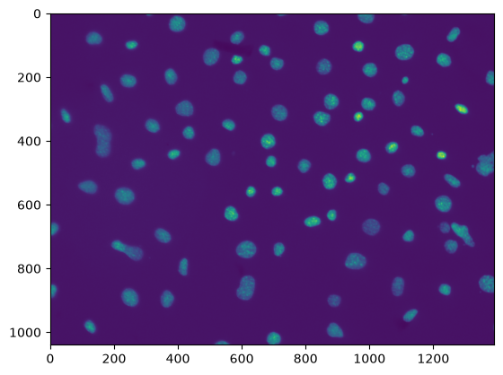
Viewing the image with `matplotlib`#

There are other ways we can view an image in Python. Another common way is to use the pyplot module of a library called matplotlib to plot the image. This way of viewing the image is very different from the ndv viewer, as the resulting image plot is not interactive.

Library Module Name	Description	How to import it	PyPi Link	Documentation Link
`pyplot`	Module within matplotlib library that creates static visualizations	`import matplotlib.pyplot`	matplotlib	matplotlib.pyplot

matplotlib contains lots of different functionality, most of which we will not be using in this course. To view an image, we just need to use the pyplot module of matplotlib. We can selectively import this portion of the overall library in two different ways:

from matplotlib import pyplot # option 1
import matplotlib.pyplot # option 2

Option 2 is more commonly used. For typing simplicity, we can use an alias when we import:

import matplotlib.pyplot as plt

To use plt now to plot our image, we write:

plt.imshow(image)

✍️ Exercise: Use `matplotlib` to view the image `raw_image`#

Don’t forget to import what you need!

import matplotlib.pyplot as plt

plt.imshow(raw_image)

<matplotlib.image.AxesImage at 0x7f87205983e0>

../../_images/6aaba3836b9a3d4bae18d66657e2d02bade4728b6386544c8eb8915e4939ff27.png

Viewing an image’s shape#

You can access many helpful image properties using Python, including an image’s shape. For a single 2D image, the image shape refers to rows and columns dimensions of the image in units of pixels. The shape is returned as (rows, columns), which corresponds to (y, x) in a 2D image.

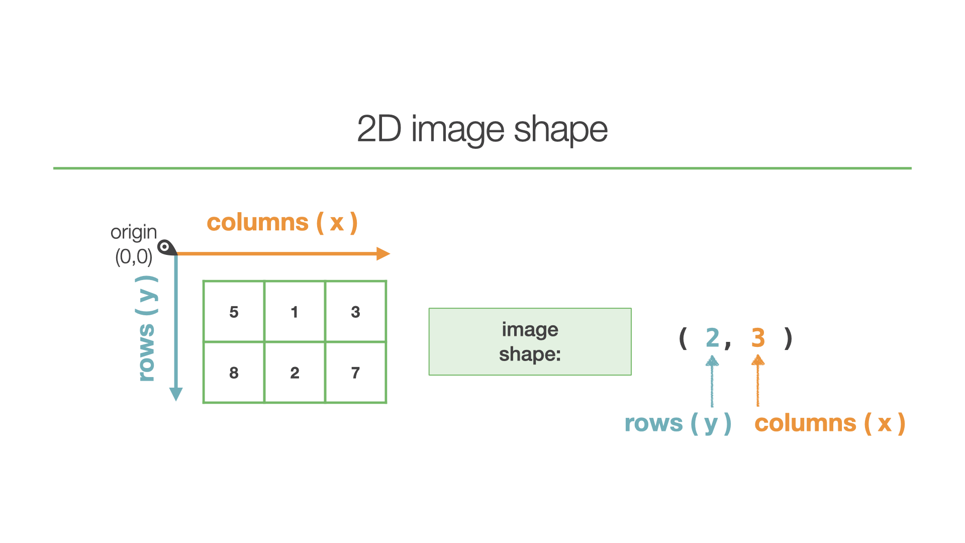
You can access an image’s shape with the following code, where image is the variable assigned to the read image file:

image.shape

Viewing an image’s dtype#

Another image property you can access using Python is an image’s dtype. An image’s dtype will specify the image bit depth, which defines the range of possible intensity values in the image.

You can access an image’s dtype with the following code:

image.dtype

Viewing an image’s type#

In the last notebook, we learned about Python’s standard data types and structures. We used the built-in function type() to check what type of data an object is. We can again apply this type() function to our image to check its type.

✍️ Exercise: Print your image’s shape, dtype, and type#

print(raw_image.shape)
print(raw_image.dtype)
print(type(raw_image))

(1040, 1392)
uint16
<class 'numpy.ndarray'>

1. Introduction to NumPy Arrays#

Concept#

A numpy array is an external data structure that is the most common representation of images in Python. Numpy is pronounced “num-pie” and stands for Numerical Python. A numpy array holds numeric data, one example is images! numpy lets us compute on and manipulate images quickly.

`numpy` is an external Python library#

Since numpy is an external Python library, you will need to import it to take advantage of numpy array functionality. The entire library contains a wide range of tools, only some of which will be covered in the course.

Name	Description	How to import it	PyPi Link	Documentation Link
`numpy`	Fundamental package for scientific computing with Python, particularly because it provides an N-dimensional array	`import numpy`	numpy	numpy

How a 2D image is organized in a `numpy` array#

Let’s consider the following simple 2D image:

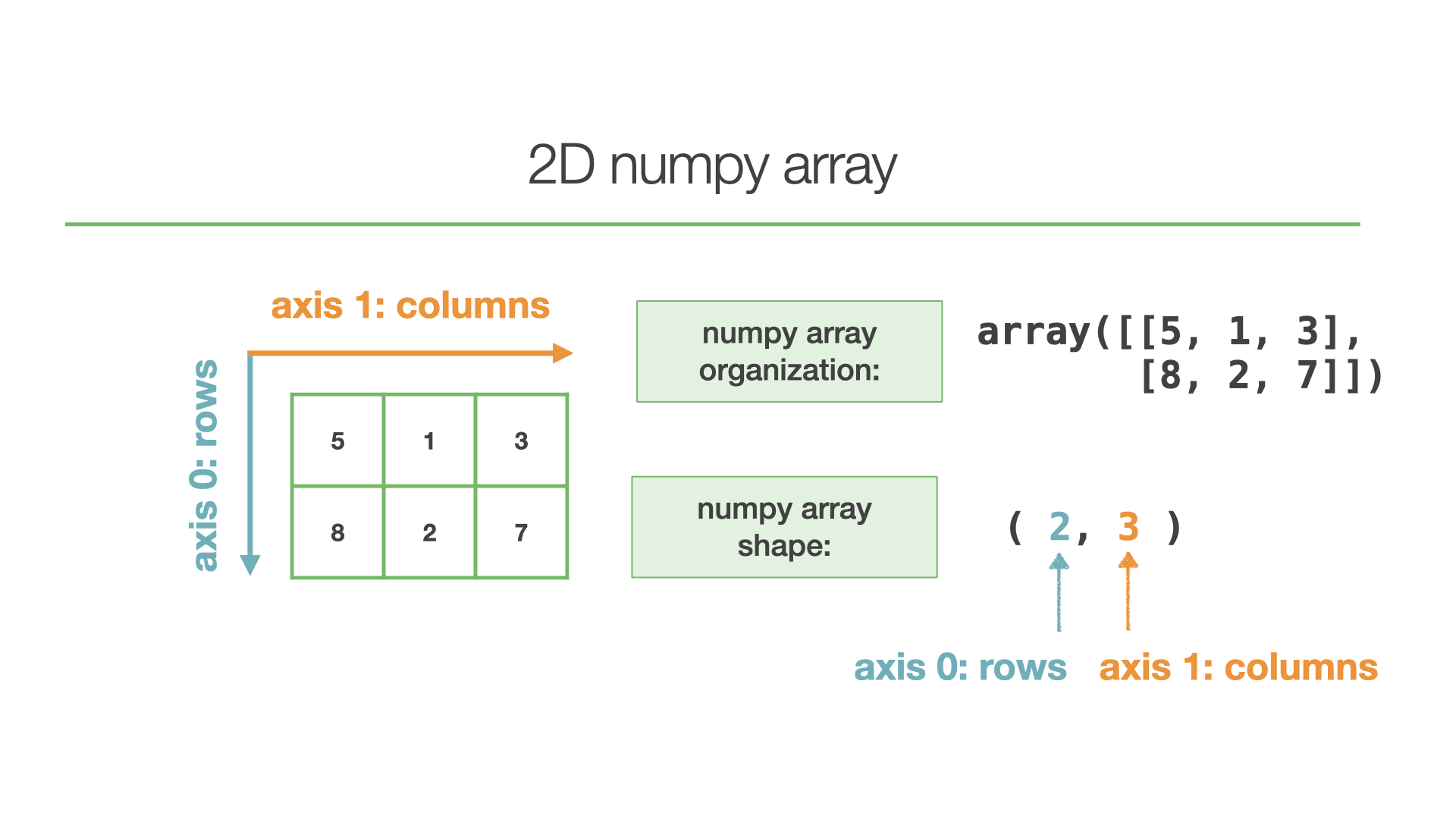
This 2D image spans two dimensions: it contains 2 rows of pixels and 3 columns of pixels. A numpy array views these two dimensions as two axes, where the first axis is the row dimension (axis 0) and the second axis is the column dimension (axis 1).

Below is how this simple 2D image is represented as a numpy array

numpy.array([[5, 1, 3],
       [8, 2, 7]])

How to view an image as a numpy array#

While ndv and matplotlib.pyplot allow us to view an image with the intensity values mapped to color, we can also view an image as a numpy array. We can do this by simply printing the variable name.

Let’s first import numpy!

✍️ Exercise: Import `numpy`#

# Note that we use the alias np to refer to the numpy library
import numpy as np

📓 Example: Run the cell to view an image as a numpy array#

print(raw_image)

[[179 184 188 ... 190 192 193]
 [200 194 189 ... 204 197 205]
 [203 203 204 ... 202 208 208]
 ...
 [218 213 224 ... 207 210 215]
 [221 217 216 ... 210 211 213]
 [217 223 222 ... 204 207 210]]

`numpy` array indexing#

We can access elements in a 2D numpy array using indexing, just as we did with the other data structures we learned about. Since we are working with a 2D array, we will have 2 indices to specify, one for each axis.

If we again consider our simple 2D image:

and it’s corresponding numpy array representation:

simple_image = numpy.array([[5, 1, 3],
                            [8, 2, 7]])

We can index the bottom left element in the array, 8, by specifying it’s index along axis 0 (2nd row), then along axis 1 (1st column):

simple_image[1, 0]

As usual with Python, a numpy array will start indexing for each axis at 0.

Now let’s get some practice with indexing numpy arrays!

✍️ Exercise: Guess the output before running the code!#

# Note: we imported numpy as np
simple_image = np.array([[0, 1, 2], [3, 4, 5], [6, 7, 8]])

print(simple_image[2, 2])

✍️ Exercise: Guess the output before running the code!#

# Note: we imported numpy as np
simple_image = np.array([[0, 1, 2], [3, 4, 5], [6, 7, 8]])

print(simple_image[1, 2])

✍️ Exercise: Guess the output before running the code!#

# Note: we imported numpy as np
simple_image = np.array([[0, 1, 2], [3, 4, 5], [6, 7, 8]])

print(simple_image[1, 0])

✍️ Exercise: Print the intensity value of the pixel in the top left corner of `raw_image`#

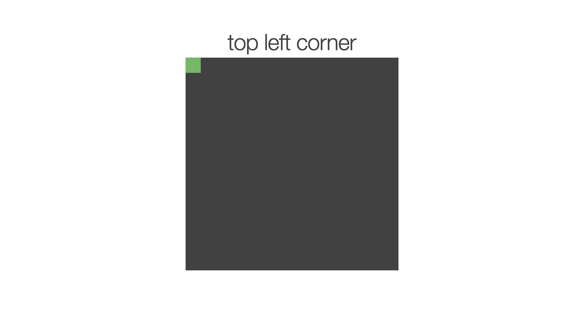
print(raw_image[0, 0])

✍️ Exercise: Print the intensity value of the pixel in the top right corner of `raw_image`#

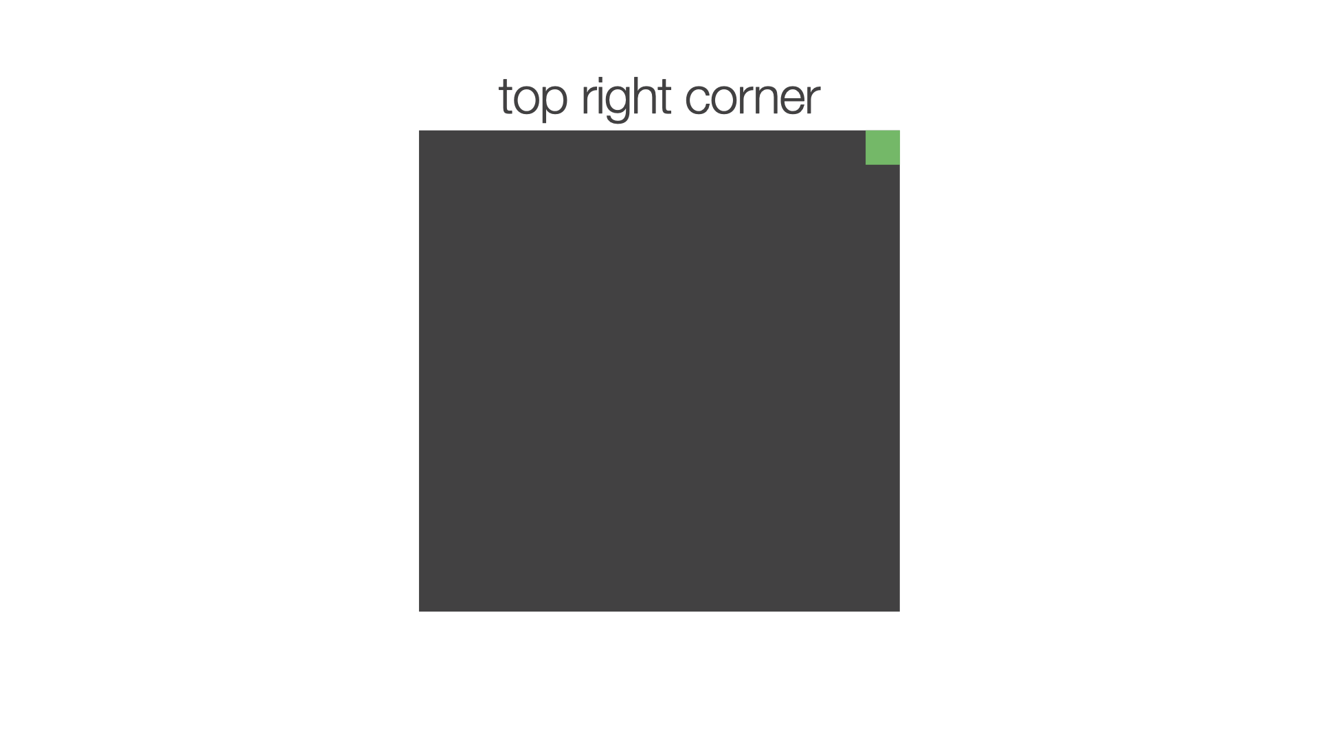
# Determine how many total columns are in the image
tot_columns = raw_image.shape[1]

# The last column index is the total number of columns minus 1 (since indexing starts at 0)
last_col_index = tot_columns - 1

# Print the top right corner pixel intensity value
print(raw_image[0, last_col_index])

✍️ Exercise: Print the intensity value of the pixel in the bottom right corner of `raw_image`#

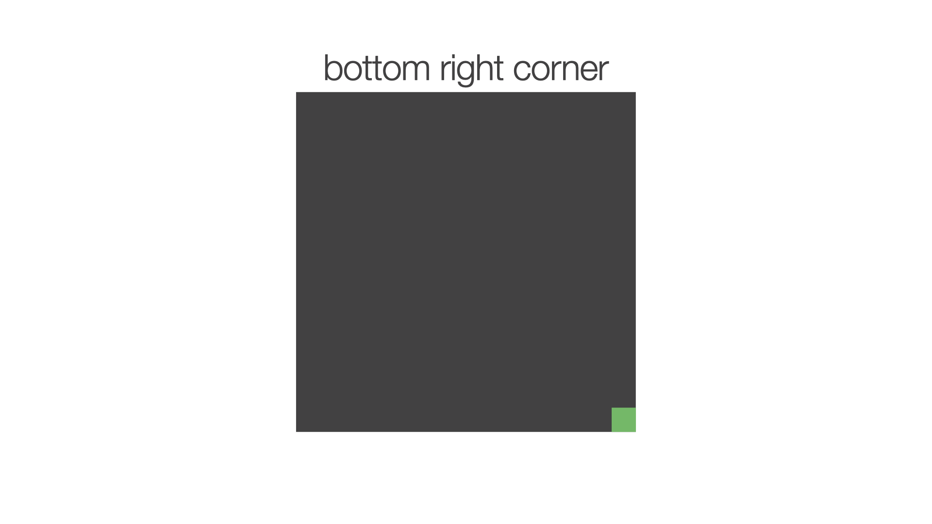
# Determine how many total rows & columns are in the image
tot_rows = raw_image.shape[0]
tot_columns = raw_image.shape[1]

# The last column index is the total number of columns minus 1 (since indexing starts at 0)
last_row_index = tot_rows - 1
last_col_index = tot_columns - 1

# Print the bottom right corner pixel intensity value
print(raw_image[last_row_index, last_col_index])

Accessing an entire row or column of a `numpy` array#

We can also access pixels across an entire row or column of a 2D image.

Accessing an entire row#

To access pixels across an entire row, we would specify the target row’s index along axis 0, and then collect all columns across it. In Python, we can specify we want all columns across a row in a few ways:

target_row = 1 # let's grab the second row in the image
image[target_row, :] # use : for the axis 1 index to collect all columns
image[target_row] # not specify a second index at all; if only one index is supplied, it applies to axis 0

Note: If only 1 index is provided for a numpy array, then Python applies that supplied index to axis 0 of the array. This is done regardless of how many dimensions the numpy array has.

Accessing an entire column#

To access pixels across an entire column, we would specify the target column and then collect all rows across it. We can write that in a few different ways as well:

target_column = 3 # let's grab the fourth column in the image
image[:, target_column] # use : for the axis 0 index to collect all rows

Now you give it a try!

✍️ Exercise: Print the first row of pixel values in `raw_image`#

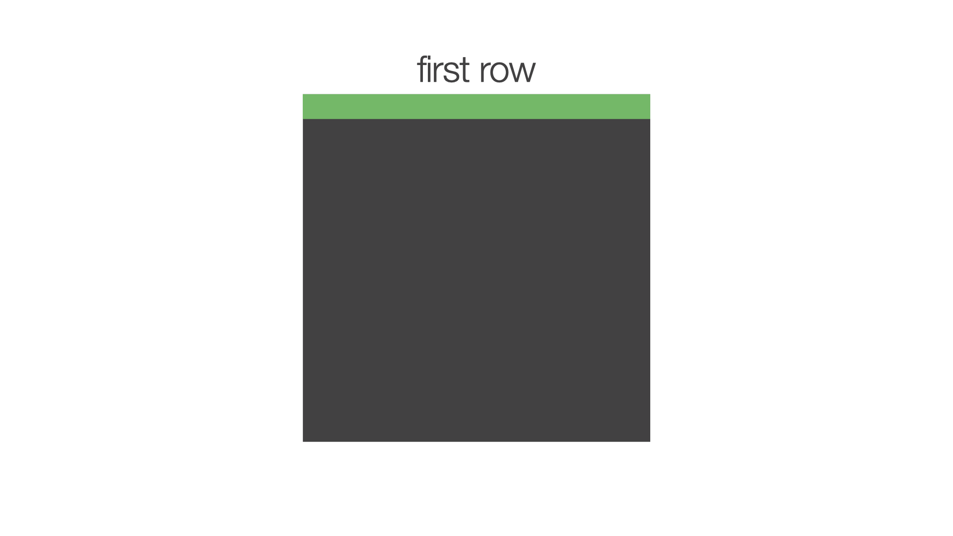
# option 1
print(raw_image[0, :])

# option 2
print(raw_image[0])

[179 184 188 ... 190 192 193]
[179 184 188 ... 190 192 193]

✍️ Exercise: Print the first column of pixel values in `raw_image`#

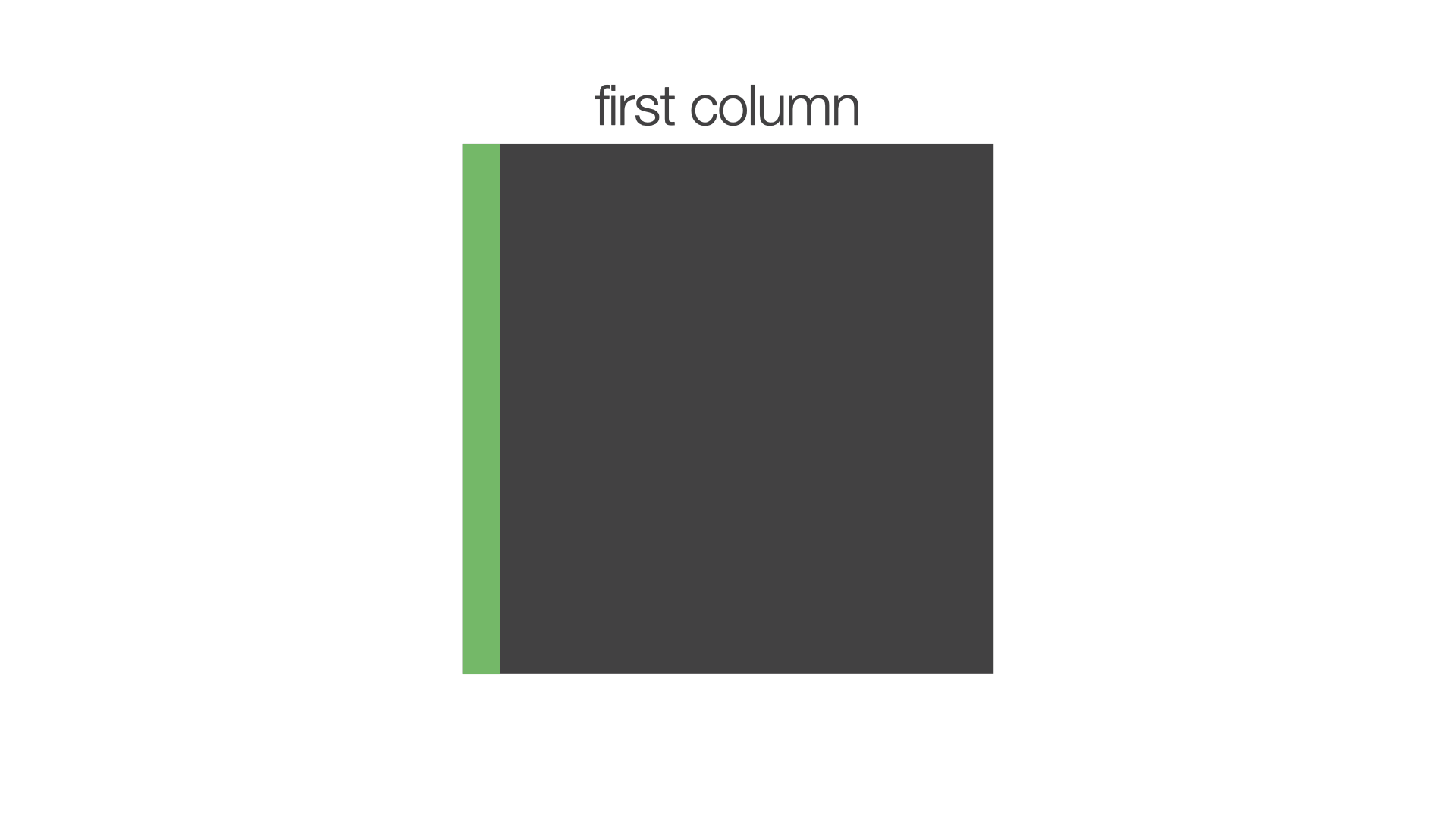
print(raw_image[:, 0])

[179 200 203 ... 218 221 217]

✍️ Exercise: Print the middle row of pixel values in `raw_image`#

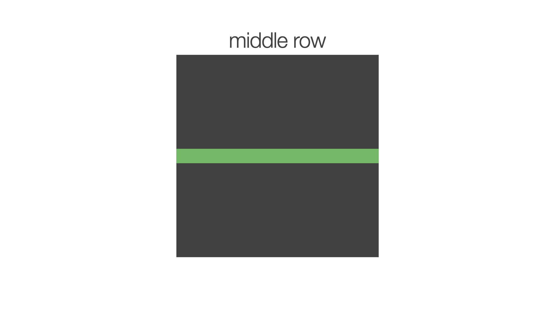
# Determine how many total rows are in the image
tot_rows = raw_image.shape[0]

# Determine the middle row index
middle_row_index = tot_rows // 2

# Print the middle row pixel intensity values
print(raw_image[middle_row_index, :])  # option 1
print(raw_image[middle_row_index])  # option 2

[223 228 223 ... 212 221 216]
[223 228 223 ... 212 221 216]

How to access pixel statistics from a numpy array#

numpy has functions that enable easy access of common pixel statistics across an entire numpy array, including the minimum, maximum, and mean. In the context of a fluorescence image, accessing these pixel statistics would inform you of the minimum, maximum, and mean intensity value, respectively.

Statistic	Description	How to use it
Minimum	Returns the minimum pixel value in the image	`image.min()`
Maximum	Returns the maximum pixel value in the image	`image.max()`
Mean	Returns the mean pixel value in the image	`image.mean()`

Now you give it a try! Go ahead and use numpy functionality to access pixel statistics for raw_image.

✍️ Exercise: Print the minimum, maximum, and mean intensity value of `raw_image`#

print(raw_image.min())  # Min pixel value
print(raw_image.max())  # Max pixel value
print(raw_image.mean())  # Average pixel value

161
1224
247.86391398651637

Note: Providing no arguments into the () of these functions leads to Python calculating these statistics across the entire ENTIRE numpy array (all axes). As we will learn in the next section, some numpy arrays will contain more than 2 axes, so calculating these statistics across all axes may not be appropriate.

2. Multidimensional Images#

Concept#

So far we have been discussing numpy arrays in the context of individual 2D images. However, numpy arrays can also be applied to multidimensional images. Common examples of multidimensional fluorescence images include z-stacks, time lapses, multiple fluorescence channels, etc. In each of these examples, an additional dimension is created to individual 2D images with x and y dimensions.

How a 3D image set is organized in a `numpy` array#

Let’s consider the following simple 3D image set containing 4 identical images:

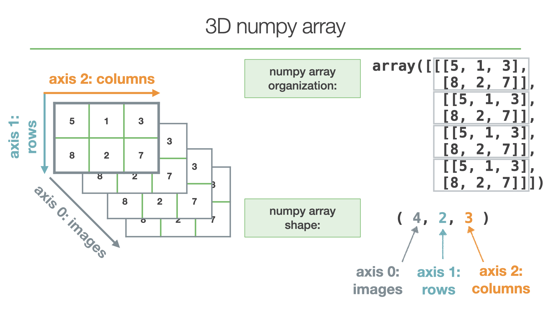
This 3D image set spans 3 dimensions: it contains 4 images, each with 2 rows of pixels and 3 columns of pixels. Just as with individual 2D images, a numpy array views these 3 dimensions as 3 axes, where the first axis is the image dimension (axis 0), the second axis is the row dimension of a given image (axis 1), and the third axis is the column dimension of a given image (axis 2).

Below is how this simple 3D image is represented as a numpy array

numpy.array([[[5, 1, 3],
             [8, 2, 7]], 
             [[5, 1, 3],
             [8, 2, 7]],
             [[5, 1, 3],
             [8, 2, 7]],
             [[5, 1, 3],
             [8, 2, 7]]])

✍️ Exercise: Print the shape of the “multichannel.tif” image to determine how many fluorescence channels it has#

Don’t forget to read the image!

image_path = r"../../_static/images/python4bia/multichannel.tif"
multichannel = tiff.imread(image_path)
print(multichannel.shape)

(2, 1040, 1392)

How to view a multidimensional image#

The simplest way to view a multidimensional image in Python is to use ndv, just as you did before with the individual 2D image.

✍️ Exercise: Use `ndv` to view the multichannel image#

ndv.imshow(multichannel)

snapshot

How to access individual images from a multidimensional image#

We can use indexing to access individual images in a multidimensional image.

What we want to do is specify the target image’s index along axis 0, and then collect all rows and columns across the image. In Python, we can specify we want all rows and columns across the target image in 2 ways:

target_image = 1 # let's grab the second image within the multidimensional image

# option 1
image_set[target_image, :, :] # use : for the axis 1 and 2 indices to collect all rows and columns

# option 2
image_set[target_image] # if only one index is supplied, it applies to axis 0

Now you give it a try!

✍️ Exercise: Use `matplotlib` to view the first channel of the “multichannel.tif” image file#

target_image = 0  # grab the first image within the multichannel image
channel_1 = multichannel[target_image, :, :]  # option 1 for indexing the first channel
channel_1 = multichannel[target_image]  # option 2 for indexing the first channel

plt.imshow(channel_1)

<matplotlib.image.AxesImage at 0x7f86cc3f26f0>

Image projections#

Z-stacks are a common example of multidimensional images in fluorescence microscopy. Z-stacks contain 2D images collected at different z planes to sample a 3D volume. One way to simplify viewing these 3D images is to collapse the data down to 2D using image projections.

Below are examples of common image projections used in fluorescence microscopy and their corresponding numpy functions. You can refer to this numpy documentation page for more details about the functions.

Type of Projection	Function	What it does along an axis	Example projection (`axis=0`)
Maximum Intensity Projection	`np.max`	Takes the maximum value	`mip = np.max(stack, axis=0)`
Minimum Intensity Projection	`np.min`	Takes the minimum value	`min_proj = np.min(stack, axis=0)`
Sum Projection	`np.sum`	Takes the sum	`sum_proj = np.sum(stack, axis=0)`
Average Intensity Projection	`np.mean`	Takes the arithmetic mean	`mean_proj = np.mean(stack, axis=0)`
Standard Deviation Projection	`np.std`	Takes the standard deviation	`sigma_map = np.std(stack, axis=0)`
Variance Projection	`np.var`	Takes the variance	`var_map = np.var(stack, axis=0)`

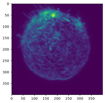
✍️ Exercise: Use `matplotlib` to display the maximum intensity projection of the “zstack.tif” image file#

Don’t forget to read the image file!

image_path = r"../../_static/images/python4bia/zstack.tif"
z_stack = tiff.imread(image_path)
mip = np.max(z_stack, axis=0)
plt.imshow(mip)

<matplotlib.image.AxesImage at 0x7f86cc011130>

../../_images/cf80fd5958bb032197ce3b111ba3d852a54c93721af38debe5c23f7112c881ed.png

3. Saving Images#

Concept#

With tifffile, we can also save output files using the function imwrite().

Saving Output Files#

To save files using imwrite(), we must specify two things:

The file path the image will be saved to, which ends with a specified file name
The data: the image you want to save!

Here’s how we can write the code to save an image output_image:

import tifffile as tiff # this would be at the beginning of the code, and only specified once
output_path = "/Users/edelase/bobiac/results/output_image.tif" # full file path including the file name we want to save
tiff.imwrite(output_path, data=output_image)

Here, tiff.imwrite is provided with 2 required inputs:

output_path is the file path the image will be saved to, which ends with a specified file name
data=output_image is a specification for the image data being saved

tiff.imwrite() will use these two inputs to output a tiff file of output_image saved to the folder specified in output_path.

✍️ Exercise: Save the maximum intensity projection of the z-stack using `tifffile`#

output_path = "path/to/output/directory/mip.tif"
tiff.imwrite(output_path, data=mip)

---------------------------------------------------------------------------
FileNotFoundError                         Traceback (most recent call last)
Cell In[25], line 2
      1 output_path = "path/to/output/directory/mip.tif"
----> 2 tiff.imwrite(output_path, data=mip)

File ~/work/bobiac-book/bobiac-book/.venv/lib/python3.12/site-packages/tifffile/tifffile.py:1507, in imwrite(file, data, mode, bigtiff, byteorder, kind, imagej, ome, shaped, append, shape, dtype, photometric, planarconfig, extrasamples, volumetric, tile, rowsperstrip, bitspersample, compression, compressionargs, predictor, subsampling, jpegtables, iccprofile, colormap, description, datetime, resolution, resolutionunit, subfiletype, software, metadata, extratags, contiguous, truncate, align, maxworkers, buffersize, returnoffset)
   1503             and not truncate
   1504             and compression in {None, 0, 1, 'NONE', 'None', 'none'}
   1505         )
   1506 
-> 1507     with TiffWriter(
   1508         file,
   1509         mode=mode,
   1510         bigtiff=bigtiff,

File ~/work/bobiac-book/bobiac-book/.venv/lib/python3.12/site-packages/tifffile/tifffile.py:1888, in TiffWriter.__init__(self, file, mode, bigtiff, byteorder, append, kind, imagej, ome, shaped)
   1884         self._ifdindex = 0
   1885         self._omexml = None
   1886         self._storedshape = None
   1887 
-> 1888         self._fh = FileHandle(file, mode=mode, size=0)
   1889         if append:
   1890             self._fh.seek(0, os.SEEK_END)
   1891         else:

File ~/work/bobiac-book/bobiac-book/.venv/lib/python3.12/site-packages/tifffile/tifffile.py:12751, in FileHandle.__init__(self, file, mode, name, offset, size)
  12747         self._offset = -1 if offset is None else offset
  12748         self._size = -1 if size is None else size
  12749         self._close = True
  12750         self._lock = contextlib.nullcontext()
> 12751         self.open()
  12752         assert self._fh is not None

File ~/work/bobiac-book/bobiac-book/.venv/lib/python3.12/site-packages/tifffile/tifffile.py:12771, in FileHandle.open(self)
  12767                 msg = f'invalid mode {self._mode}'
  12768                 raise ValueError(msg)
  12769             self._file = os.path.realpath(self._file)
  12770             self._dir, self._name = os.path.split(self._file)
> 12771             self._fh = open(  # noqa: SIM115
  12772                 self._file, self._mode, encoding=None
  12773             )
  12774             self._close = True

FileNotFoundError: [Errno 2] No such file or directory: '/home/runner/work/bobiac-book/bobiac-book/content/03_digital_images_intro/path/to/output/directory/mip.tif'

4. Visualizing Multiple Images#

Concept#

So far we have been using ndv to view multidimensional images. We can also use matplotlib.pyplot, but doing so would involve plotting multiple images. One way we can do this is by organizing each image as a subplot within an overall figure.

How a figure can be organized with `matplotlib.pyplot`#

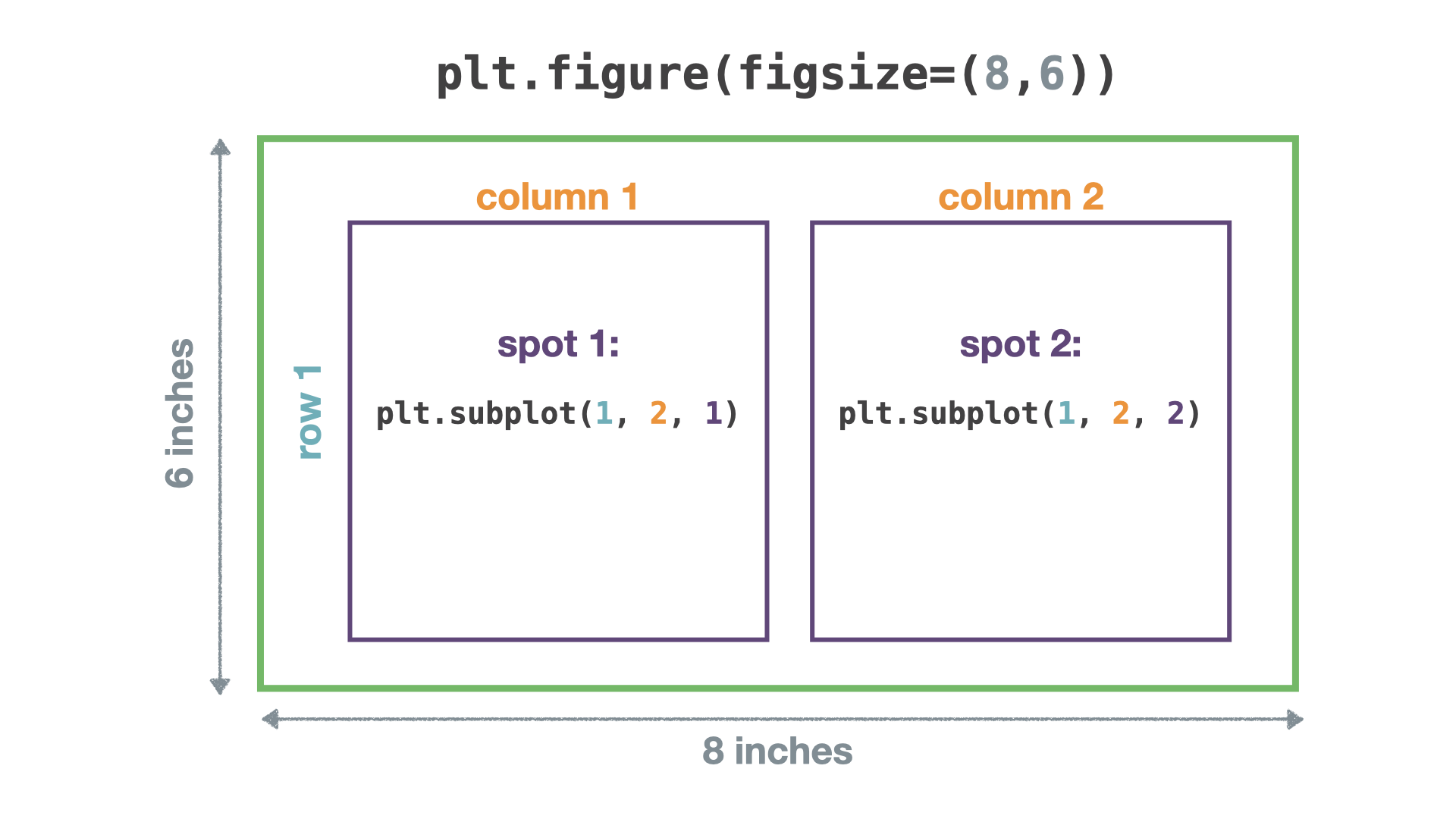
Creating a figure#

Using matplotlib.pyplot, we can create a 8 inch x 6 inch figure by writing the following:

import matplotlib.pyplot as plt

# Create a figure
plt.figure(figsize=(8, 6))

Filling the figure with subplots, each containing images#

The code above creates an empty figure. We will now need to fill it with subplots containing images. We can use the subplot() function to create a subplots organized in a total number of rows and columns, and select a specific spot to put an image into:

plt.subplot(tot_rows, tot_columns, specific_spot)

To fill the figure with 2 subplots organized next to each other, we would want to have 1 row and 2 columns. We would therefore write the following:

# Select the first spot and plot an image into it
plt.subplot(1, 2, 1) # (1 row, 2 columns, first spot)
plt.imshow(img_1)

# Select the second spot and plot an image into it
plt.subplot(1, 2, 2) # (1 row, 2 columns, second spot)
plt.imshow(img_2)

Displaying the final figure#

Once you have added the images to the figure, you can display it with the following:

# Show the plot
plt.show()

Caution: Using matplotlib.pyplot.subplot() is not the only way that you can plot multiple images in a figure with matplotlib.pyplot. Ironically, another common way to plot multiple images in a figure is with matplotlib.pyplot.subplots(). While both accomplish the same final result, the second option uses a different indexing system to add items to each subplot.

✍️ Exercise: Use `matplotlib` to display each channel of the “multichannel.tif” image file, side by side#

# read the multichannel image
image_path = r"../../_static/images/python4bia/multichannel.tif"
multichannel = tiff.imread(image_path)

# check the shape of the multichannel image
print(
    multichannel.shape
)  # we see that it's a 2 channel image with dimensions 1392x1040 px

# create a figure with 2 subplots, one for each channel
plt.figure(figsize=(8, 6))  # 8 inches wide, 6 inches tall

# channel 1 in the first subplot position
plt.subplot(1, 2, 1)  # 1 row, 2 columns, first subplot
plt.imshow(multichannel[0])  # channel 1 in the first subplot

# channel 2 in the second subplot position
plt.subplot(1, 2, 2)  # 1 row, 2 columns, second subplot
plt.imshow(multichannel[1])  # channel 2 in the second subplot

# show the plot
plt.show()

Figure Aesthetics#

matplotlib.pyplot has additional settings you can use to edit the look of these figures. Below are a few key examples of aspects you can edit, although many more options can be found in the documentation.

Removing axis labels#

If you do not want to display the axis number labels on the sides of images, you can turn them off by writing plt.axis("off") for each subplot after plotting the image:

# Create a figure
plt.figure(figsize=(8, 6))

# First subplot
plt.subplot(1, 2, 1)
plt.imshow(img_1)
plt.axis("off")  # Turn off axis labels

# Second subplot
plt.subplot(1, 2, 2)
plt.imshow(img_2)
plt.axis("off")  # Turn off axis labels

Changing the lookup table (LUT)#

You can change the LUT of the image display by specifying a colormap for each subplot. Color map options can be found in this documentation page. If the colormap is not specified, matplotlib.pyplot defaults to using the viridis colormap.

You can specify the colormap cmap for a subplot by including it when you plot the image

plt.subplot(1, 2, 1)
plt.imshow(img_1, cmap="gray") # will use the gray colormap to plot img_1

Adjusting image brightness & contrast#

You can also change the color mapping of the image to its minimum and maximum intensity values, rather than to the minimum and maximum of the image bit depth. Doing so will help you view features in the image more clearly.

You can specify the minimum vmin and maximum vmax value of the color mapping by including it when you plot the image:

plt.subplot(1, 2, 1)
plt.imshow(img_1, cmap="gray", vmin=img_1.min(), vmax=img_1.max()) # adjust to the min and max of img_1

Fitting the subplots in the figure#

When you create a figure with subplots, you specify the figure size but not individual subplot sizes. If the figure size is too small to fit individual subplots, you can run into situations where the axis labels, among other things for each image, will overlap. matplotlib.pyplot has a layout setting called constrained layout, which you can use to fit plots within your figure cleanly. Constrained layout automatically adjusts subplots so that decorations like tick labels do not overlap.

You can specify you want to use constrained layout by specifying it when you define the figure:

plt.figure(figsize=(8, 6), layout="constrained")  # use constrained layout

✍️ Exercise: Edit your “multichannel.tif” plot above to display each image with a different colormap, adjusted to the min and max of the image. Hide the axis labels, and use constrained layout.#

# create a figure with 2 subplots, one for each channel
plt.figure(figsize=(8, 6), layout="constrained")  # 8 inches wide, 6 inches tall

# channel 1 in the first subplot position
plt.subplot(1, 2, 1)  # 1 row, 2 columns, first subplot
plt.imshow(
    multichannel[0],
    cmap="Greens",
    vmin=multichannel[0].min(),
    vmax=multichannel[0].max(),
)
plt.axis("off")  # turn off axes labels for the first subplot

# channel 2 in the second subplot position
plt.subplot(1, 2, 2)  # 1 row, 2 columns, second subplot
plt.imshow(
    multichannel[1],
    cmap="Purples",
    vmin=multichannel[1].min(),
    vmax=multichannel[1].max(),
)
plt.axis("off")  # turn off axes labels for the second subplot

# show the plot
plt.show()

Visualizing multiple images with `ndv`#

ndv also has display options we can set. We can specify the LUT for each channel and view the composite, or overlaid image of channels.

Viewing the composite image#

We can view the composite image of a multichannel image file by specifying the channel_mode:

ndv.imshow(image, channel_mode="composite")

Specifying channel LUTs#

We can also specify each channel’s LUT by referring to the channel’s index:

ndv.imshow(
    image, 
    channel_mode="composite", 
    luts = {0:{"cmap":"green"}, 1: {"cmap": "magenta"}}
)

5. BONUS: Reading Proprietary File Types#

Concept#

In many cases, images you acquire from commercial microscope acquisition software will have proprietary file types (e.g., .nd2 for Nikon NIS Elements, .czi for Zeiss ZEN Blue, etc.). tifffile will fail to read these files because they are not tiff files. Instead, you can use the Python library bffile to read these file types.

Library Name	Description	How to import it	PyPi Link	Documentation Link
`bffile`	Reads and stores a wide variety of commercial file formats (e.g., .nd2, .czi, .lif, etc.) as np.arrays	`import bffile`	bffile	bffile

In order to read an image with bffile, we will need to import it, and then provide it with the image’s path.

import bffile
image_path = r"path/to/file"
image = bffile.imread(image_path)

bffile.imread() will use that image_path you inputted to find your file and read it. It will then return the read file.

✍️ Exercise: Use `bffile` to read the “2D_image.nd2” image and assign it to the variable `nd2_image`. Then, print its shape.#

Don’t forget to import bffile!

import bffile

image_path = r"../../_static/images/python4bia/2D_image.nd2"
nd2_image = bffile.imread(image_path)
print(nd2_image.shape)

How bffile organizes an image’s `numpy` array#

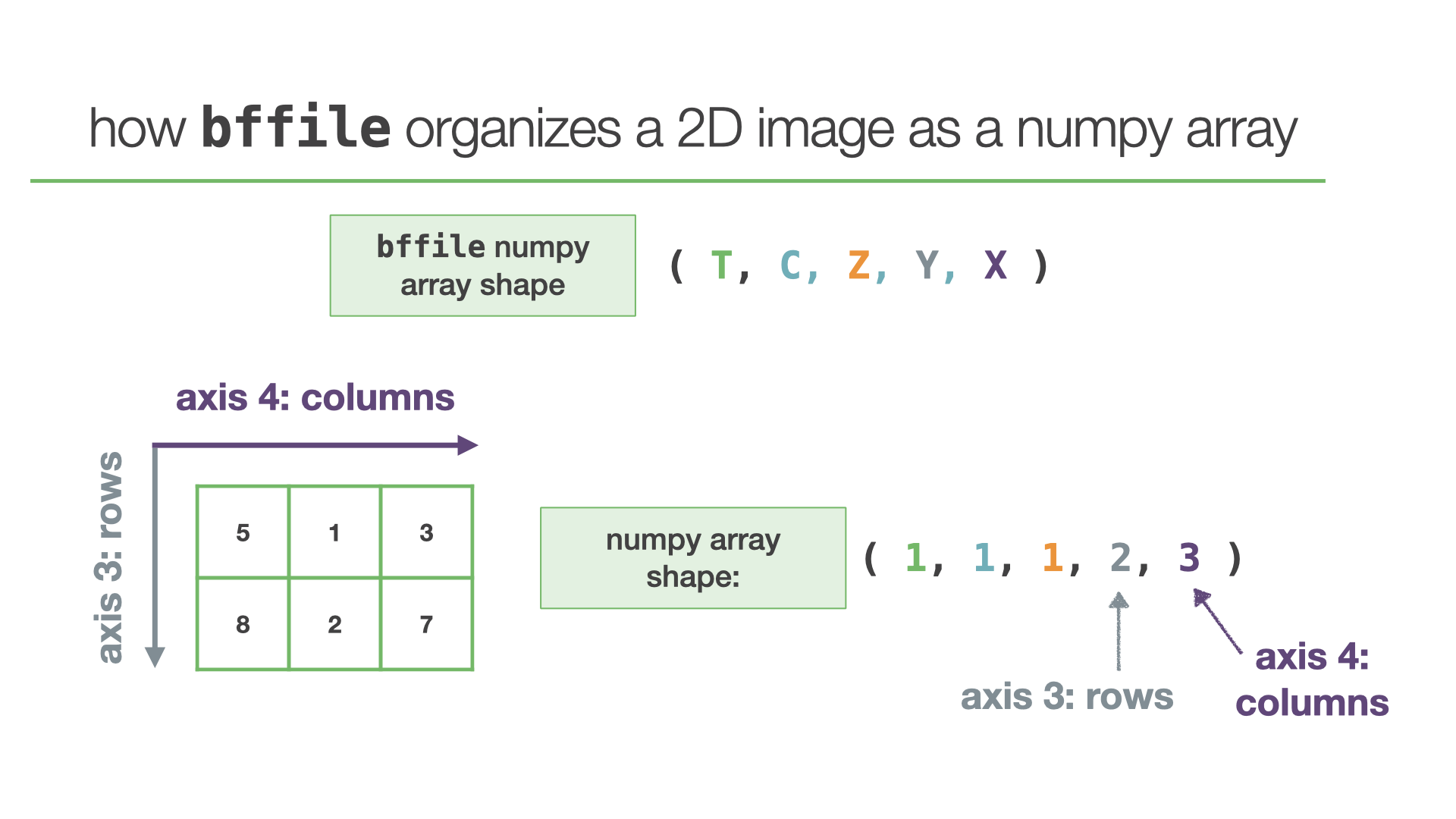
When bffile.imread() reads an image, it always organizes the image as a numpy array with a shape (T, C, Z, Y, X), where: T = Time Point Images C = Channel Images Z = z Slice Images Y = Rows in an Image X = Columns in an Image

If the image does not have time points, channels, or z slices, the length of that axis will be 1. Consider again our simple 2D image. If we use bffile.imread() to load this image, its numpy array will be organized as a 5D array.

Using `numpy.squeeze()` to drop unnecessary axes#

At times, it can be clunky to carry around those extra dimensions if they are not relevant to the given image. We can use numpy.squeeze() to get rid of specific axes that have a length of 1.

Library Module Name	Description	How to use it	Documentation Link
`numpy.squeeze()`	Remove axes of length one from a `numpy` array	`numpy.squeeze(array, axis=axis)`	numpy.squeeze()

To use numpy.squeeze(), we provide the numpy array. We can also provide a specific axis number to drop. If no axis is provided, numpy.squeeze() will drop any axes with length 1. Here’s an example:

numpy.squeeze(image, axis = 0) # drop only the first axis from the numpy array image
numpy.squeeze(image) # drop any axes with length 1 from the numpy array image

Note: numpy.squeeze() will raise an error if an axis is selected with shape entry greater than one.

✍️ Exercise: Drop unnecessary axes from `nd2_image`. Print its shape to confirm the change.#

Note: Remember that we imported numpy with the alias np

# check image shape
print(nd2_image.shape)  # we see T, C, Z are all 1 and can be dropped

# Option 1: Drop T, C, and Z axes all at once
nd2_image_nTCZ = np.squeeze(nd2_image)
print(nd2_image_nTCZ.shape)  # we now have (2044, 2048)

# Option 2: Drop T, C, and Z axes one at a time
# drop T axis
nd2_image_nT = np.squeeze(nd2_image, axis=0)
print(nd2_image_nT.shape)  # we now have (1, 1, 2044, 2048)

# drop C axis
nd2_image_nC = np.squeeze(nd2_image_nT, axis=0)
print(nd2_image_nC.shape)  # we now have (1, 2044, 2048)

# drop Z axis
nd2_image_nZ = np.squeeze(nd2_image_nC, axis=0)
print(nd2_image_nZ.shape)  # we now have (2044, 2048)

Next Steps#

Congratulations for making it to the end of this lesson! You have now started learning how to work with images in Python! However, just as with syntax, there is always more to learn when it comes to mastering a programming language and mindset. Below is another resource we recommend to review concepts and build upon your new-found knowledge.

1. BoBiAC Exercises: Working with Bioimages

2. Reviewing Images & Pixels with Python: Pete Bankhead’s Introduction to Bioimage Analysis Book is a self-paced beginner resource that covers many of the core topics introduced in this lesson within the “Introducing Images” section.

Working with Bioimages in Python

Contents

Working with Bioimages in Python#

Overview#

0. Reading an Image#

Concept#

Specifying your file’s path#

Loading an image#

✍️ Exercise: Use tifffile to read the “2D_image.tif” image and assign it to the variable raw_image.#

Viewing the image with ndv#

✍️ Exercise: Use ndv to view the image raw_image#

Viewing the image with matplotlib#

✍️ Exercise: Use matplotlib to view the image raw_image#

Viewing an image’s shape#

Viewing an image’s dtype#

Viewing an image’s type#

✍️ Exercise: Print your image’s shape, dtype, and type#

1. Introduction to NumPy Arrays#

Concept#

numpy is an external Python library#

How a 2D image is organized in a numpy array#

How to view an image as a numpy array#

✍️ Exercise: Import numpy#

📓 Example: Run the cell to view an image as a numpy array#

numpy array indexing#

✍️ Exercise: Guess the output before running the code!#

✍️ Exercise: Guess the output before running the code!#

✍️ Exercise: Guess the output before running the code!#

✍️ Exercise: Print the intensity value of the pixel in the top left corner of raw_image#

✍️ Exercise: Print the intensity value of the pixel in the top right corner of raw_image#

✍️ Exercise: Print the intensity value of the pixel in the bottom right corner of raw_image#

Accessing an entire row or column of a numpy array#

Accessing an entire row#

Accessing an entire column#

✍️ Exercise: Print the first row of pixel values in raw_image#

✍️ Exercise: Print the first column of pixel values in raw_image#

✍️ Exercise: Print the middle row of pixel values in raw_image#

How to access pixel statistics from a numpy array#

✍️ Exercise: Print the minimum, maximum, and mean intensity value of raw_image#

2. Multidimensional Images#

Concept#

How a 3D image set is organized in a numpy array#

✍️ Exercise: Print the shape of the “multichannel.tif” image to determine how many fluorescence channels it has#

How to view a multidimensional image#

✍️ Exercise: Use ndv to view the multichannel image#

How to access individual images from a multidimensional image#

✍️ Exercise: Use matplotlib to view the first channel of the “multichannel.tif” image file#

Image projections#

✍️ Exercise: Use matplotlib to display the maximum intensity projection of the “zstack.tif” image file#

3. Saving Images#

Concept#

Saving Output Files#

✍️ Exercise: Save the maximum intensity projection of the z-stack using tifffile#

4. Visualizing Multiple Images#

Concept#

How a figure can be organized with matplotlib.pyplot#

Creating a figure#

Filling the figure with subplots, each containing images#

Displaying the final figure#

✍️ Exercise: Use matplotlib to display each channel of the “multichannel.tif” image file, side by side#

Figure Aesthetics#

Removing axis labels#

Changing the lookup table (LUT)#

Adjusting image brightness & contrast#

Fitting the subplots in the figure#

✍️ Exercise: Edit your “multichannel.tif” plot above to display each image with a different colormap, adjusted to the min and max of the image. Hide the axis labels, and use constrained layout.#

Visualizing multiple images with ndv#

Viewing the composite image#

Specifying channel LUTs#

5. BONUS: Reading Proprietary File Types#

Concept#

✍️ Exercise: Use bffile to read the “2D_image.nd2” image and assign it to the variable nd2_image. Then, print its shape.#

How bffile organizes an image’s numpy array#

Using numpy.squeeze() to drop unnecessary axes#

✍️ Exercise: Drop unnecessary axes from nd2_image. Print its shape to confirm the change.#

Next Steps#

✍️ Exercise: Use `tifffile` to read the “2D_image.tif” image and assign it to the variable `raw_image`.#

✍️ Exercise: Use `ndv` to view the image `raw_image`#

Viewing the image with `matplotlib`#

✍️ Exercise: Use `matplotlib` to view the image `raw_image`#

`numpy` is an external Python library#

How a 2D image is organized in a `numpy` array#

✍️ Exercise: Import `numpy`#

`numpy` array indexing#

✍️ Exercise: Print the intensity value of the pixel in the top left corner of `raw_image`#

✍️ Exercise: Print the intensity value of the pixel in the top right corner of `raw_image`#

✍️ Exercise: Print the intensity value of the pixel in the bottom right corner of `raw_image`#

Accessing an entire row or column of a `numpy` array#

✍️ Exercise: Print the first row of pixel values in `raw_image`#

✍️ Exercise: Print the first column of pixel values in `raw_image`#

✍️ Exercise: Print the middle row of pixel values in `raw_image`#

✍️ Exercise: Print the minimum, maximum, and mean intensity value of `raw_image`#

How a 3D image set is organized in a `numpy` array#

✍️ Exercise: Use `ndv` to view the multichannel image#

✍️ Exercise: Use `matplotlib` to view the first channel of the “multichannel.tif” image file#

✍️ Exercise: Use `matplotlib` to display the maximum intensity projection of the “zstack.tif” image file#

✍️ Exercise: Save the maximum intensity projection of the z-stack using `tifffile`#

How a figure can be organized with `matplotlib.pyplot`#

✍️ Exercise: Use `matplotlib` to display each channel of the “multichannel.tif” image file, side by side#

Visualizing multiple images with `ndv`#

✍️ Exercise: Use `bffile` to read the “2D_image.nd2” image and assign it to the variable `nd2_image`. Then, print its shape.#

How bffile organizes an image’s `numpy` array#

Using `numpy.squeeze()` to drop unnecessary axes#

✍️ Exercise: Drop unnecessary axes from `nd2_image`. Print its shape to confirm the change.#