Measurement Pipeline

Measurement Pipeline#

# /// script
# requires-python = ">=3.10"
# dependencies = [
#     "matplotlib",
#     "numpy",
#     "scikit-image",
#     "scipy",
#     "tifffile",
#     "imagecodecs",
#     "pandas",
#     "seaborn",
#     "bobiac_tools @ git+https://github.com/bobiac/bobiac-tools.git"
# ]
# ///

Overview#

In this notebook, we will run through a full measurement pipeline.

Our data are two images of cells stained with phalloidin (F-actin). One image is from an untreated control and one from a drug tretment. Our question is: Does the drug change F-actin abundance and/or cell size?

To find out we will learn how to extract single cell properties using the scikit-image library. Moreover, we will learn how to use the pandas library for data handling. Lastly we will brifly introduce seaborn for simple plotting and visualisation.

The data for this exercise is the same as used for the classic segmentation, deep learning segmentation and spot detection exercises and can be downloaded here. From the previous segmentation exercises you should have a collection of labelled masks for the cells. If not you can download them from here.

Importing libraries#

from pathlib import Path

import matplotlib.pyplot as plt
import numpy as np
import skimage
import tifffile
from bobiac_tools import overlay_labels

Load and Display Image and Label Mask#

First we load and display our control image and segmentation. We will walk through how to set up the measurements first and then apply the same strategy to the image of the drug treated cells.

We visualise the image and the segmentation with the overlay function. Hint: if you just want to plot the image use the overlay function with just the image.

image_path = Path(
    "../../_static/images/quant/01_measurement_quantification/images/F01_202.tif"
)
label_path = Path(
    "../../_static/images/quant/01_measurement_quantification/masks/F01_202_cell_labels.tif"
)

image = tifffile.imread(image_path)[1, :, :]
labeled_mask = tifffile.imread(label_path)

overlay_labels(image, labeled_mask)

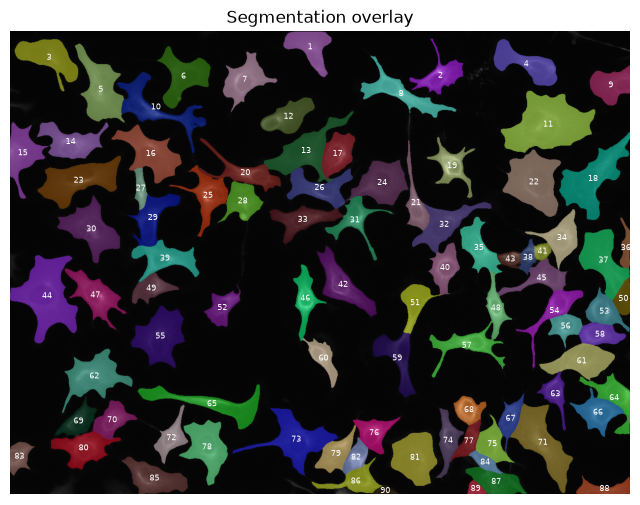
../../_images/5557e32cc722f31ecc381dee2a5740d9996d43f2d65ac2ebb19aec8f0a849083.png

Before we use the segmentation to measure, we need to remove all objects that touch the border, since they are likely not fully in the field of view and therefore not measurable.

# remove objects that touch the border of the image
labeled_mask = skimage.segmentation.clear_border(labeled_mask)

overlay_labels(image, labeled_mask, alpha=0.2)

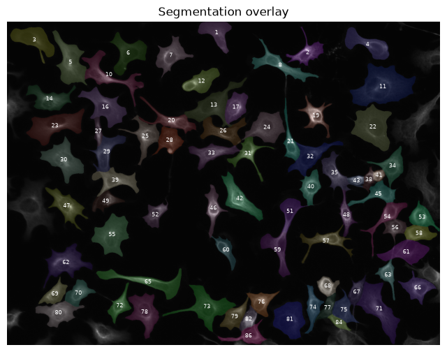
../../_images/16d4acf9e9e86033af2ff6aa5688af254c1089be7b9916ba0af1678e1d49828b.png

As we learned before, the labeled mask is a picture the same size of the raw image that has pixel value 0 for the background and a unique integer > 0 for each segmented object this value we call an objects index. Here, we plotted each segmented object in a different color together with its index.

We can directly access specific objects in our label mask by addressing them using their index.

# create an image that contains only the mask of the indexed object
index = 42

# note that == creates a boolean mask by comparing each pixel to the index value, resulting in True for pixels belonging to the object and False for all other pixels
idx_object = labeled_mask == index

# Plot the extracted cell image
plt.figure(figsize=(6, 6))
plt.imshow(idx_object, cmap="gray")
plt.title(f"Object {index}")
plt.axis("off")
plt.show()

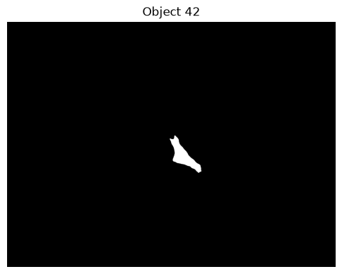
../../_images/02df317aac98a140c236312c4190d55510d4bd0b005994fb1af0c49c0e7a3087.png

This new image we obtained is a boolean mask with value False for background and True for the object with the index we specified.

To verify that this is indeed a binary mask, we can query for the minimum and maximum value using the np.min() and np.max() functions:

print("Data type:", idx_object.dtype)

print("Min value:", np.min(idx_object))
print("Max value:", np.max(idx_object))

Data type: bool
Min value: False
Max value: True

Manual Extraction of Properties#

Now we can use this mask to measure properties of the object such as its area or the fluorescence intensity of that region in the raw image (i.e. the intensity of the cell).

Area measurement#

To measure the area of the object we can make use of the fact that the boolean mask is False or 0 outside of the object and True or 1 inside it.

# counts the number of True pixels, which corresponds to the area of the object in pixels
object_area = np.sum(idx_object)
print(f"Area of object {index}: {object_area} pixels")

Area of object 42: 7395 pixels

To convert the area in pixels to µm, we can multiply it with the squared pixel size in µm. Here we assume that one pixels has the size 0.325 µm.

pixel_size = 0.325  # µm
object_area_um = object_area * (pixel_size**2)
print(f"Area of object {index}: {object_area_um} um^2")

Area of object 42: 781.0968750000001 um^2

Intensity measurement#

To measure the objects intensity, we can use the boolean mask to index our raw image.

# Extract the intensity values of the pixels that belong to this nucleus from the original image
# This uses the boolean mask to index into the original image
object_intesities = image[idx_object]

# Print the intensity values and its variable type and shape
print("Type of object_intesities:", type(object_intesities))
print("Shape of object_intesities:", object_intesities.shape)
print(f"Intensity values of object {index}: {object_intesities}")

Type of object_intesities: <class 'numpy.ndarray'>
Shape of object_intesities: (7395,)
Intensity values of object 42: [217 191 214 ... 206 224 197]

We can then calculate the mean intensity using the np.mean() function:

object_mean_intensity = np.mean(object_intesities)
print(f"Mean intensity of object {index}: {object_mean_intensity}")

Mean intensity of object 42: 886.4260987153482

✍️ Exercise: Measure area, basic intensity features for all nuclei in the dataset#

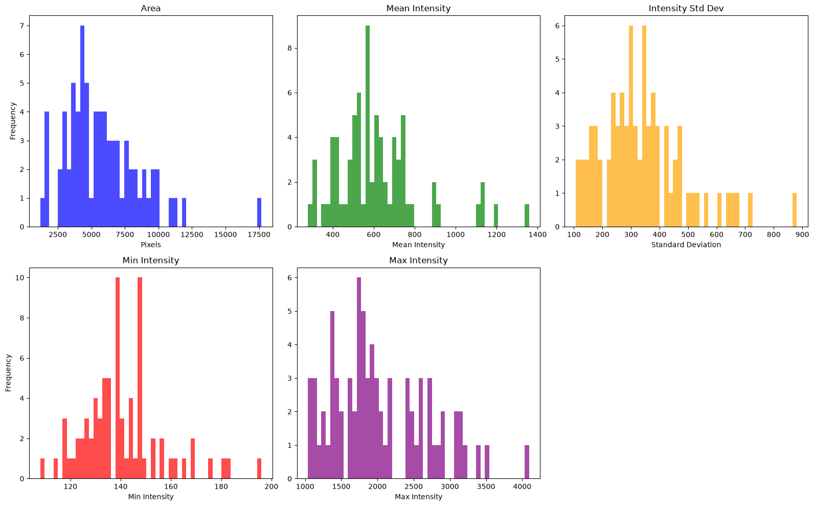
In this exercise, we want to measure for each object in our segmentation mask its area, its mean intensity, the variabilty of its intensity (via standard deviation), and its minimum and maximum intensity values. For this, you can follow these steps:

Create an empty list for each feature (e.g. area_list).
Write a for loop that iterates over all object indices in the segmentation mask.
For each iteration measure all features (useful functions are np.std, np.min, np.max) and store them in the corresponding list.
Plot each feature as a histogram using plt.hist.

# measure area and intensity statistics for all nuclei in the labeled mask
object_indices = np.unique(labeled_mask)
object_indices = object_indices[object_indices != 0]  # skip background

area_list = []
mean_intensity_list = []
std_intensity_list = []
min_intensity_list = []
max_intensity_list = []

for obj_id in object_indices:
    mask = labeled_mask == obj_id
    intensities = image[mask]

    area_list.append(np.sum(mask))
    mean_intensity_list.append(np.mean(intensities))
    std_intensity_list.append(np.std(intensities))
    min_intensity_list.append(np.min(intensities))
    max_intensity_list.append(np.max(intensities))

# plot histograms for each feature
plt.figure(figsize=(16, 10))

plt.subplot(2, 3, 1)
plt.hist(area_list, bins=50, color="blue", alpha=0.7)
plt.title("Area")
plt.xlabel("Pixels")
plt.ylabel("Frequency")

plt.subplot(2, 3, 2)
plt.hist(mean_intensity_list, bins=50, color="green", alpha=0.7)
plt.title("Mean Intensity")
plt.xlabel("Mean Intensity")

plt.subplot(2, 3, 3)
plt.hist(std_intensity_list, bins=50, color="orange", alpha=0.7)
plt.title("Intensity Std Dev")
plt.xlabel("Standard Deviation")

plt.subplot(2, 3, 4)
plt.hist(min_intensity_list, bins=50, color="red", alpha=0.7)
plt.title("Min Intensity")
plt.xlabel("Min Intensity")
plt.ylabel("Frequency")

plt.subplot(2, 3, 5)
plt.hist(max_intensity_list, bins=50, color="purple", alpha=0.7)
plt.title("Max Intensity")
plt.xlabel("Max Intensity")

plt.tight_layout()
plt.show()

../../_images/c9c28bb870668e676947b17f8926eef8ce742519338d563d84d69da40e986689.png

Automated Extraction of Properties#

The skimage.measure module from scikit-image provides efficient tools for measuring properties of labeled image regions, extracting both morphological and intensity-based features for every object in a single call.

A central function in this module is regionprops_table:

Parameters:

label_image — A 2D or 3D integer array where each unique non-zero value identifies a distinct object.
intensity_image (optional) — The corresponding grayscale image, required for intensity-based measurements.
properties — A list of property names to measure and compute.

For example:

skimage.measure.regionprops_table(label_image, intensity_image=image, properties=["area", "intensity_mean"])

Returns:

A dict mapping each property name to an array of values, one per labeled object.

The table below summarizes commonly used properties:

Measurement	Description
area	Number of pixels in the object (size)
perimeter	Approximate boundary length
eccentricity	Elongation of the shape (0 = circle, 1 = line segment)
solidity	Ratio of object area to its convex hull area
orientation	Angle of the major axis relative to the horizontal
intensity_mean	Mean pixel intensity within the region
intensity_std	Standard deviation of pixel intensities within the region
intensity_max	Maximum pixel intensity within the region
intensity_min	Minimum pixel intensity within the region
image_intensity	Pixel values cropped to the object’s bounding box
centroid	Center of mass coordinates
bbox	Bounding box coordinates
coords	List of coordinates of all pixels (y, x)

A full list of all measurable properties can be found in the regionprops documentation.

Use regionprops_table to extract measurements from labeled_mask and image:

# compute label, area, and mean intensity for each object in the label mask
props = skimage.measure.regionprops_table(
    labeled_mask, image, ["label", "area", "intensity_mean"]
)
print("Datatype:", type(props))
print("Keys in props:", list(props.keys()))
print(" ")
print("All features for all objects:\n", props)

Datatype: <class 'dict'>
Keys in props: ['label', 'area', 'intensity_mean']
 
All features for all objects:
 {'label': array([ 1,  2,  3,  4,  5,  6,  7,  8, 10, 11, 12, 13, 14, 16, 17, 19, 20,
       21, 22, 23, 24, 25, 26, 27, 28, 29, 30, 31, 32, 33, 34, 35, 38, 39,
       40, 41, 42, 43, 45, 46, 47, 48, 49, 51, 52, 53, 54, 55, 56, 57, 58,
       59, 60, 61, 62, 63, 65, 66, 67, 68, 69, 70, 71, 72, 73, 74, 75, 76,
       77, 78, 79, 80, 81, 82, 84, 86]), 'area': array([ 5634.,  4728.,  7677.,  6824.,  9638.,  7597.,  6457.,  6623.,
        8089., 17676.,  5623.,  9464.,  6870.,  8757.,  5192.,  4511.,
        5498.,  3704., 11958., 10928.,  8255.,  5922.,  6221.,  1790.,
        4905.,  5894.,  9128.,  4602.,  7087.,  5809.,  5392.,  5493.,
        1726.,  6322.,  4469.,  1193.,  7395.,  1526.,  4674.,  4392.,
        6731.,  3363.,  3606.,  4110.,  3619.,  4218.,  4654.,  9771.,
        3111.,  5339.,  3853.,  5943.,  3227.,  7514.,  9025.,  3037.,
        7956.,  5224.,  3094.,  3038.,  3670.,  4349., 11120.,  3664.,
        9978.,  4029.,  4096.,  4163.,  2607.,  8142.,  4289.,  6577.,
        8947.,  2622.,  1669.,  4207.]), 'intensity_mean': array([ 422.20429535,  764.30160745,  279.3688941 ,  433.45720985,
        492.97157087,  316.81084639,  537.64565588,  609.06688812,
        526.76832736,  390.69025798,  553.85630446,  373.71544801,
        532.89315866,  417.78508622,  647.29776579, 1116.23852804,
        714.18188432,  786.19195464,  303.40500084,  407.13707906,
        506.70769231,  606.00776765,  474.93473718,  744.92793296,
        525.03547401,  579.88361045,  497.56047327,  710.19100391,
        428.97911669,  707.7982441 ,  576.90504451,  643.90842891,
        741.65701043,  567.59569756,  674.03110316, 1358.36378877,
        886.42609872, 1132.65661861,  577.76358579,  884.67827869,
        639.71267271,  921.25007434,  501.10094287,  420.6836983 ,
        573.33075435,  695.35751541,  643.3036098 ,  392.24347559,
        617.98264224,  740.96328901,  627.92681028,  514.39475013,
        499.53455222,  346.96167155,  569.14725762,  747.78696082,
        530.85947712,  591.60490046,  606.84033613, 1126.83838051,
        573.26376022,  563.71280754,  467.48417266,  650.75409389,
        395.45319703,  612.6840407 ,  533.88110352,  725.59788614,
        590.39470656,  492.20854827,  563.03520634,  693.65333739,
        314.86509445, 1197.80167811,  753.53025764,  716.49037319])}

regionprops_table creates a dictionary where the keys are the names of the properties and the values are numpy arrays of the measurements of the properties for all objects in the label mask. We can access all area measurements like this: props['area'] and an object-specific area measurement like this: props['area'][index] with index being e.g. 0 for the first object. The order of objects is the same across all property arrays.

print("Area for all objects:\n", props["area"])
print()
# we use index-1 because the label IDs start at 1, but list indexing starts at 0
print(f"Area for object {index}:", props["area"][index - 1])

Area for all objects:
 [ 5634.  4728.  7677.  6824.  9638.  7597.  6457.  6623.  8089. 17676.
 9464.  6870.  8757.  5192.  4511.  5498.  3704. 11958. 10928.
 5922.  6221.  1790.  4905.  5894.  9128.  4602.  7087.  5809.
 5493.  1726.  6322.  4469.  1193.  7395.  1526.  4674.  4392.
 3363.  3606.  4110.  3619.  4218.  4654.  9771.  3111.  5339.
 5943.  3227.  7514.  9025.  3037.  7956.  5224.  3094.  3038.
 4349. 11120.  3664.  9978.  4029.  4096.  4163.  2607.  8142.
 6577.  8947.  2622.  1669.  4207.]

Area for object 42: 3363.0

As you can see, we get the same area value we obtained manually before.

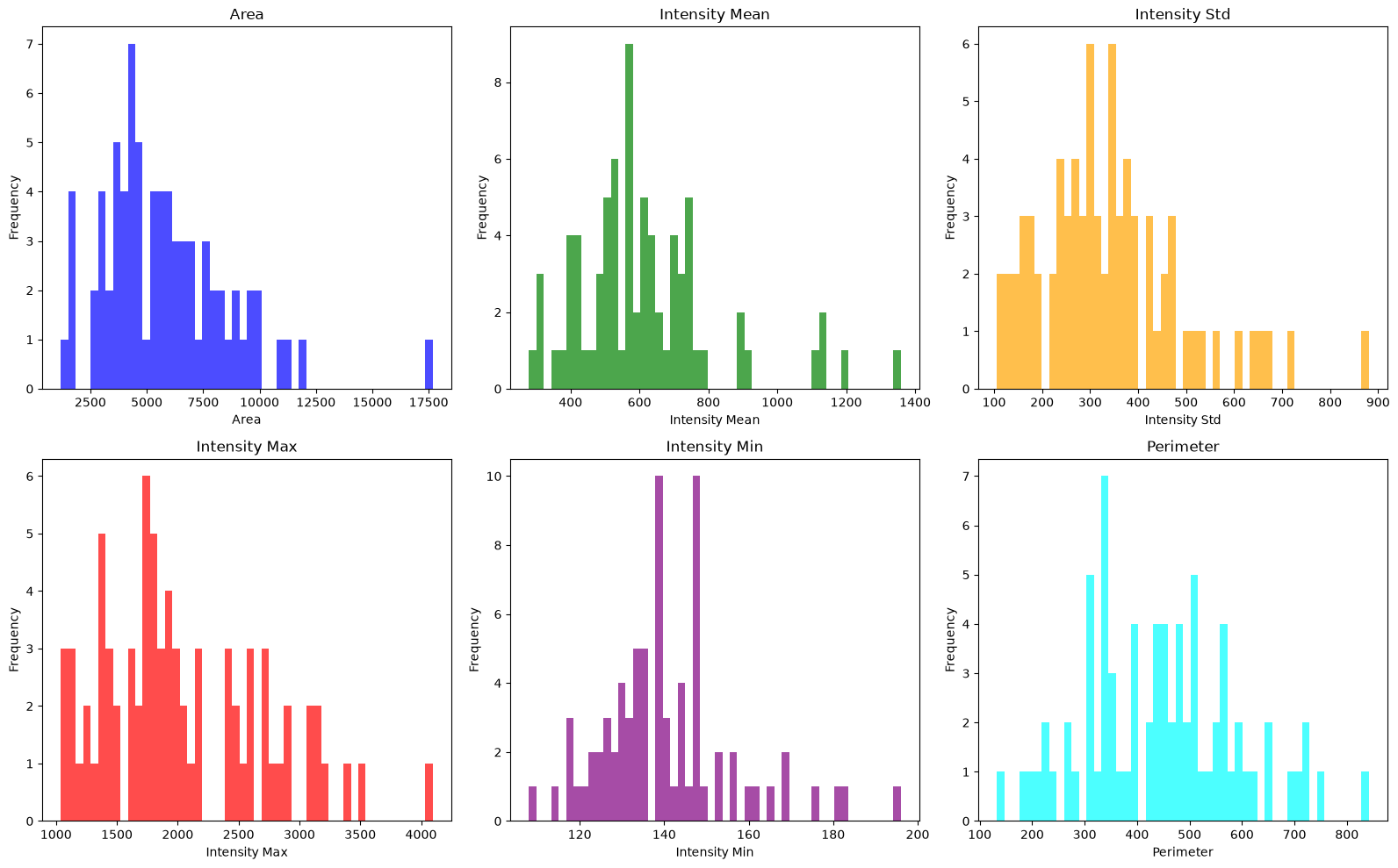
✍️ Exercise: Use `regionprops_table` to measure basic features of all nuclei#

In this exercise, we repeat the exercise above using regionprops_table instead of looping over each object. Measure area, intensity_mean, intensity_std, intensity_max, intensity_min, and (this one is new) perimeter. For that you can:

Use regionprops with the appropriate properties.
Use plt.hist to plot a histogram for each property. (You can use a for loop for that if you want to be efficient.)

Note how much less code you have to write compared with the previous exercise.

Bonus: think about how you would implement the perimeter property manually.

properties = [
    "area",
    "intensity_mean",
    "intensity_std",
    "intensity_max",
    "intensity_min",
    "perimeter",
]

props_basic = skimage.measure.regionprops_table(
    labeled_mask, intensity_image=image, properties=properties
)

list_colors = ["blue", "green", "orange", "red", "purple", "cyan"]

plt.figure(figsize=(16, 10))
for i, prop in enumerate(properties, start=1):
    plt.subplot(2, 3, i)
    plt.hist(props_basic[prop], bins=50, color=list_colors[i - 1], alpha=0.7)
    plt.title(prop.replace("_", " ").title())
    plt.xlabel(prop.replace("_", " ").title())
    plt.ylabel("Frequency")

plt.tight_layout()
plt.show()

../../_images/0ffbbe474d198671073f4b58ff86c97c15e160a2cfcd76618160d625d34db83d.png

Tables -> `pandas.DataFrame`#

Using lists, dictionaries and np.arrays for data analysis works fine, but is a little bit clunky. Here, we introduce a more streamlined and straightforward method for storing and accessing your data. We use the pandas package which is centred around the DataFrame object, an intuitive 2D table that allows basic plotting, labelling of rows, columns and conditional indexing as well as table operations such as melt and pivot and summary statistics like mean or std.

This is a brief interlude before we return to comparing our control and drug treated cells. It will be worth it in the end.

We start by importing pandas and creating a new DataFrame variable.

import pandas as pd

properties = [
    "area",
    "intensity_mean",
    "intensity_std",
    "intensity_max",
    "intensity_min",
    "perimeter",
]
props = skimage.measure.regionprops_table(
    labeled_mask, intensity_image=image, properties=properties
)

df = pd.DataFrame(props)
print(df)

      area  intensity_mean  intensity_std  intensity_max  intensity_min  \
 5634.0      422.204295     198.333981         1118.0          132.0   
 4728.0      764.301607     523.274140         3509.0          138.0   
 7677.0      279.368894     125.690020         1069.0          118.0   
 6824.0      433.457210     254.054528         1445.0          120.0   
 9638.0      492.971571     267.211757         1934.0          123.0   
..     ...             ...            ...            ...            ...   
6577.0      693.653337     335.493382         1762.0          147.0   
8947.0      314.865094     106.334739         1124.0          162.0   
2622.0     1197.801678     717.324747         3076.0          175.0   
1669.0      753.530258     221.434922         1388.0          196.0   
4207.0      716.490373     264.225298         1605.0          181.0   

     perimeter  
 376.877200  
 516.416306  
 502.031529  
 444.132034  
 570.535101  
..         ...  
457.546248  
392.776695  
228.350288  
205.072114  
449.339141  

[76 rows x 6 columns]

Note how tidy this format is. Individual cells are rows containing all measuremnt that relate to that cell and columns are sets of measurements for all cells.

Accessing data in `DataFrames`#

Accessing columns works similar to dictionaries: df[column] or df[[list_of_columns]].

# Print just the area column
print(df["area"])

   5634.0
   4728.0
   7677.0
   6824.0
   9638.0
       ...  
  6577.0
  8947.0
  2622.0
  1669.0
  4207.0
Name: area, Length: 76, dtype: float64

# Print area and mean intensity columns
print(df[["area", "intensity_mean"]])

      area  intensity_mean
 5634.0      422.204295
 4728.0      764.301607
 7677.0      279.368894
 6824.0      433.457210
 9638.0      492.971571
..     ...             ...
6577.0      693.653337
8947.0      314.865094
2622.0     1197.801678
1669.0      753.530258
4207.0      716.490373

[76 rows x 2 columns]

Accessing rows can be done via index using .iloc or by condition using .loc.

First we can access all the properties of the previously selected cell 42.

# again, we use index-1 to access the correct row corresponding to the object with label ID equal to index
print(df.iloc[index - 1])

area              3363.000000
intensity_mean     921.250074
intensity_std      559.656385
intensity_max     2871.000000
intensity_min      144.000000
perimeter          388.634560
Name: 41, dtype: float64

We can index conditionally based on properties. Here we select all cells with an area larger than 3000 pixels.

print(df[df["area"] > 3000])

      area  intensity_mean  intensity_std  intensity_max  intensity_min  \
 5634.0      422.204295     198.333981         1118.0          132.0   
 4728.0      764.301607     523.274140         3509.0          138.0   
 7677.0      279.368894     125.690020         1069.0          118.0   
 6824.0      433.457210     254.054528         1445.0          120.0   
 9638.0      492.971571     267.211757         1934.0          123.0   
..     ...             ...            ...            ...            ...   
8142.0      492.208548     225.113748         1723.0          139.0   
4289.0      563.035206     310.288222         1863.0          144.0   
6577.0      693.653337     335.493382         1762.0          147.0   
8947.0      314.865094     106.334739         1124.0          162.0   
4207.0      716.490373     264.225298         1605.0          181.0   

     perimeter  
 376.877200  
 516.416306  
 502.031529  
 444.132034  
 570.535101  
..         ...  
487.587878  
337.362482  
457.546248  
392.776695  
449.339141  

[69 rows x 6 columns]

To fully understand what happened there, we break this line into parts.

# this creates a boolean Series where each value is True if the corresponding row in the 'area' column is greater than 3000, and False otherwise
bool_series = df["area"] > 3000
print("boolean Series:\n", bool_series)
# then we use this boolean Series to index into the DataFrame, which returns only the rows where the condition is True, i.e., where the area is greater than 3000 pixels
print("\nFiltered DataFrame:\n", df[bool_series])

boolean Series:
    True
    True
    True
    True
    True
      ...  
   True
   True
  False
  False
   True
Name: area, Length: 76, dtype: bool

Filtered DataFrame:
       area  intensity_mean  intensity_std  intensity_max  intensity_min  \
 5634.0      422.204295     198.333981         1118.0          132.0   
 4728.0      764.301607     523.274140         3509.0          138.0   
 7677.0      279.368894     125.690020         1069.0          118.0   
 6824.0      433.457210     254.054528         1445.0          120.0   
 9638.0      492.971571     267.211757         1934.0          123.0   
..     ...             ...            ...            ...            ...   
8142.0      492.208548     225.113748         1723.0          139.0   
4289.0      563.035206     310.288222         1863.0          144.0   
6577.0      693.653337     335.493382         1762.0          147.0   
8947.0      314.865094     106.334739         1124.0          162.0   
4207.0      716.490373     264.225298         1605.0          181.0   

     perimeter  
 376.877200  
 516.416306  
 502.031529  
 444.132034  
 570.535101  
..         ...  
487.587878  
337.362482  
457.546248  
392.776695  
449.339141  

[69 rows x 6 columns]

A variety of different logical operations can be used for conditional indexing via .loc. Those include: <, >, <=, >=, ==, != (not equal to), .isin(list) (equal to any object in list), ~ (not). Morover, multiple conditions can be chained using & (and), | (or) operators (each condition has to be in () parenthesis for this). Visit the excellent pandas tutorial on selecting subsets from DataFrames for more details.

# select all rows where area is greater than 2000 pixels and mean intensity is less than 400 and print their perimeter values
filtered_df = df[(df["area"] > 2000) & (df["intensity_mean"] < 350)]
print(filtered_df)

       area  intensity_mean  intensity_std  intensity_max  intensity_min  \
  7677.0      279.368894     125.690020         1069.0          118.0   
  7597.0      316.810846     124.751047         1243.0          124.0   
11958.0      303.405001     109.566139         1173.0          108.0   
 7514.0      346.961672     147.307176         1040.0          132.0   
 8947.0      314.865094     106.334739         1124.0          162.0   

     perimeter  
 502.031529  
 486.629509  
507.972655  
432.451840  
392.776695  

# select all rows where area is exactly 12061 or 9504 pixels
filtered_df = df[df["area"].isin([12061, 9504])]
print(filtered_df)

Empty DataFrame
Columns: [area, intensity_mean, intensity_std, intensity_max, intensity_min, perimeter]
Index: []

# select all rows where the intensity is between 400 and 750
filtered_df = df[(df["intensity_mean"] >= 400) & (df["intensity_mean"] <= 750)]
print(filtered_df)

       area  intensity_mean  intensity_std  intensity_max  intensity_min  \
  5634.0      422.204295     198.333981         1118.0          132.0   
  6824.0      433.457210     254.054528         1445.0          120.0   
  9638.0      492.971571     267.211757         1934.0          123.0   
  6457.0      537.645656     309.074083         2414.0          133.0   
  6623.0      609.066888     378.843471         2428.0          135.0   
  8089.0      526.768327     416.895764         2463.0          132.0   
 5623.0      553.856304     399.380371         2585.0          127.0   
 6870.0      532.893159     342.724796         2445.0          141.0   
 8757.0      417.785086     192.811960         1760.0          136.0   
 5192.0      647.297766     386.178570         2808.0          147.0   
 5498.0      714.181884     467.629040         2493.0          147.0   
10928.0      407.137079     230.782862         2197.0          127.0   
 8255.0      506.707692     183.724106         1226.0          153.0   
 5922.0      606.007768     420.649652         2730.0          147.0   
 6221.0      474.934737     238.841292         1718.0          147.0   
 1790.0      744.927933     460.751617         2173.0          169.0   
 4905.0      525.035474     309.486280         2071.0          133.0   
 5894.0      579.883610     300.464515         1785.0          139.0   
 9128.0      497.560473     255.820633         1909.0          139.0   
 4602.0      710.191004     536.782629         2920.0          139.0   
 7087.0      428.979117     169.294201         1367.0          129.0   
 5809.0      707.798244     344.109913         1736.0          156.0   
 5392.0      576.905045     260.248557         1473.0          127.0   
 5493.0      643.908429     349.713916         2581.0          144.0   
 1726.0      741.657010     427.743292         1986.0          157.0   
 6322.0      567.595698     305.411773         1869.0          148.0   
 4469.0      674.031103     373.436235         1938.0          139.0   
 4674.0      577.763586     289.596288         2150.0          121.0   
 6731.0      639.712673     394.802939         3369.0          136.0   
 3606.0      501.100943     355.683935         1930.0          130.0   
 4110.0      420.683698     264.272849         1427.0          139.0   
 3619.0      573.330754     365.042858         2028.0          118.0   
 4218.0      695.357515     347.754417         2080.0          135.0   
 4654.0      643.303610     363.383852         1977.0          130.0   
 3111.0      617.982642     292.135334         2001.0          129.0   
 5339.0      740.963289     465.550611         2709.0          138.0   
 3853.0      627.926810     272.436370         1424.0          123.0   
 5943.0      514.394750     294.029167         1607.0          145.0   
 3227.0      499.534552     345.419554         1781.0          114.0   
 9025.0      569.147258     298.716704         1818.0          141.0   
 3037.0      747.786961     382.537518         1833.0          133.0   
 7956.0      530.859477     461.637322         2573.0          133.0   
 5224.0      591.604900     302.105757         1842.0          130.0   
 3094.0      606.840336     277.560513         1678.0          142.0   
 3670.0      573.263760     339.089447         1701.0          148.0   
 4349.0      563.712808     300.727550         1641.0          160.0   
11120.0      467.484173     234.880140         1494.0          124.0   
 3664.0      650.754094     380.256293         1739.0          153.0   
 4029.0      612.684041     335.538409         1820.0          136.0   
 4096.0      533.881104     164.492270         1125.0          130.0   
 4163.0      725.597886     432.454876         2691.0          165.0   
 2607.0      590.394707     244.040069         1353.0          138.0   
 8142.0      492.208548     225.113748         1723.0          139.0   
 4289.0      563.035206     310.288222         1863.0          144.0   
 6577.0      693.653337     335.493382         1762.0          147.0   
 4207.0      716.490373     264.225298         1605.0          181.0   

     perimeter  
 376.877200  
 444.132034  
 570.535101  
 474.931024  
 689.997041  
 841.879292  
343.605122  
508.658946  
547.529004  
311.906638  
644.038672  
563.244733  
429.676190  
588.215295  
507.043723  
226.710678  
354.569589  
472.782792  
504.516811  
620.085353  
552.635606  
456.475180  
428.753355  
433.031529  
201.095454  
532.457936  
337.427453  
442.853860  
569.103643  
307.220346  
352.498521  
315.255880  
326.605122  
575.380772  
273.929978  
725.109740  
275.994949  
459.504617  
338.190909  
611.156421  
351.078210  
727.872150  
402.132034  
335.492424  
305.433550  
311.427453  
592.085353  
364.540151  
401.948268  
344.226443  
337.119841  
274.764502  
487.587878  
337.362482  
457.546248  
449.339141  

# select all rows where the area is smaller than 10 pixels
filtered_df = df[df["area"] < 10]
print(filtered_df)

Empty DataFrame
Columns: [area, intensity_mean, intensity_std, intensity_max, intensity_min, perimeter]
Index: []

Note that if no criterion in .loc is met, we get an Empty DataFrame.

✍️ Exercise: Use `iloc` and `loc` to access specific measurements in the `DataFrame`#

In this exercise, use the iloc and loc indexers to access specific entries of df.

Print only the first ten rows.
Print all rows where the perimeter is smaller than 140 pixels.
Print all rows where the area is smaller than 1500 pixesl or the minimum intensity exceeds 0.08.
BONUS: Print the area of all rows where instensity_std is less than 100.

# 1. Print only the first ten rows
print("First ten rows:")
print(df.iloc[:10])
print("\n" + "=" * 80 + "\n")

# 2. Print all rows where the perimeter is smaller than 140 pixels
print("Rows where perimeter < 140:")
print(df[df["perimeter"] < 140])
print("\n" + "=" * 80 + "\n")

# 3. Print all rows where area is smaller than 1500 pixels OR minimum intensity exceeds 0.08
print("Rows where area < 1500 OR intensity_min > 0.08:")
print(df[(df["area"] < 1500) | (df["intensity_min"] > 0.08)])
print("\n" + "=" * 80 + "\n")

# 4. BONUS: Print the area of all rows where intensity_std is less than 100
print("Area of rows where intensity_std < 100:")
print(df[df["intensity_std"] < 100]["area"])

First ten rows:
      area  intensity_mean  intensity_std  intensity_max  intensity_min  \
 5634.0      422.204295     198.333981         1118.0          132.0   
 4728.0      764.301607     523.274140         3509.0          138.0   
 7677.0      279.368894     125.690020         1069.0          118.0   
 6824.0      433.457210     254.054528         1445.0          120.0   
 9638.0      492.971571     267.211757         1934.0          123.0   
 7597.0      316.810846     124.751047         1243.0          124.0   
 6457.0      537.645656     309.074083         2414.0          133.0   
 6623.0      609.066888     378.843471         2428.0          135.0   
 8089.0      526.768327     416.895764         2463.0          132.0   
17676.0      390.690258     175.981511         1312.0          118.0   

    perimeter  
376.877200  
516.416306  
502.031529  
444.132034  
570.535101  
486.629509  
474.931024  
689.997041  
841.879292  
652.256926  

================================================================================

Rows where perimeter < 140:
      area  intensity_mean  intensity_std  intensity_max  intensity_min  \
1193.0     1358.363789     633.460391         2927.0          182.0   

     perimeter  
133.154329  

================================================================================

Rows where area < 1500 OR intensity_min > 0.08:
      area  intensity_mean  intensity_std  intensity_max  intensity_min  \
 5634.0      422.204295     198.333981         1118.0          132.0   
 4728.0      764.301607     523.274140         3509.0          138.0   
 7677.0      279.368894     125.690020         1069.0          118.0   
 6824.0      433.457210     254.054528         1445.0          120.0   
 9638.0      492.971571     267.211757         1934.0          123.0   
..     ...             ...            ...            ...            ...   
6577.0      693.653337     335.493382         1762.0          147.0   
8947.0      314.865094     106.334739         1124.0          162.0   
2622.0     1197.801678     717.324747         3076.0          175.0   
1669.0      753.530258     221.434922         1388.0          196.0   
4207.0      716.490373     264.225298         1605.0          181.0   

     perimeter  
 376.877200  
 516.416306  
 502.031529  
 444.132034  
 570.535101  
..         ...  
457.546248  
392.776695  
228.350288  
205.072114  
449.339141  

[76 rows x 6 columns]

================================================================================

Area of rows where intensity_std < 100:
Series([], Name: area, dtype: float64)

Create new columns and math on columns#

The DataFrame format allows us to do calculations using whole columns and to save the results in new columns. This is very useful for doing calculations on the raw measurements.

Let’s measure the background intensity and subtract it from the mean intensity of all objects

# calculate bg intensity
# this calculates the mean intensity of all pixels in the original image that belong to the background (where labeled_mask == 0)
background_intensity = image[labeled_mask == 0].mean()
print("Background intensity:", background_intensity, "\n")
print(
    "Mean intensity (background-subtracted):\n",
    df["intensity_mean"] - background_intensity,
)

Background intensity: 127.24859276905134 

Mean intensity (background-subtracted):
    294.955703
    637.053015
    152.120301
    306.208617
    365.722978
         ...     
   566.404745
   187.616502
  1070.553085
   626.281665
   589.241780
Name: intensity_mean, Length: 76, dtype: float64

# We can store the background-subtracted mean intensity in a new column in the DataFrame
df["intensity_mean_bg_subtracted"] = df["intensity_mean"] - background_intensity
print(df[["intensity_mean", "intensity_mean_bg_subtracted"]])

    intensity_mean  intensity_mean_bg_subtracted
     422.204295                    294.955703
     764.301607                    637.053015
     279.368894                    152.120301
     433.457210                    306.208617
     492.971571                    365.722978
..             ...                           ...
    693.653337                    566.404745
    314.865094                    187.616502
   1197.801678                   1070.553085
    753.530258                    626.281665
    716.490373                    589.241780

[76 rows x 2 columns]

Note how intuitive this syntax is. We can also do calculations using multiple rows of the DataFrame.

Let’s calculate the difference between the maximum and minimum intensity for each object and store it in a new column called intensity_range.

df["intensity_range"] = df["intensity_max"] - df["intensity_min"]
print(df[["intensity_max", "intensity_min", "intensity_range"]])

    intensity_max  intensity_min  intensity_range
        1118.0          132.0            986.0
        3509.0          138.0           3371.0
        1069.0          118.0            951.0
        1445.0          120.0           1325.0
        1934.0          123.0           1811.0
..            ...            ...              ...
       1762.0          147.0           1615.0
       1124.0          162.0            962.0
       3076.0          175.0           2901.0
       1388.0          196.0           1192.0
       1605.0          181.0           1424.0

[76 rows x 3 columns]

✍️ Exercise: Create a couple of new columns#

Create a column called cell_id containing integer values that correspond to the value of the object in the label mask.
Create a column called sum_intensity that contains the sum of all pixel intensities (mean intensity * number of pixels).
BONUS: Create a column called circularity that is 1 if an object is perfectly circular and goes towards 0 otherwise.

df["cell_id"] = object_indices
df["intensity_sum"] = df["intensity_mean"] * df["area"]
df["circularity"] = 4 * np.pi * df["area"] / (df["perimeter"] ** 2)

# this prints the first 5 rows of the DataFrame, showing the new columns we created
print(df[["cell_id", "intensity_sum", "circularity"]].head())

   cell_id  intensity_sum  circularity
      1      2378699.0     0.498456
      2      3613618.0     0.222786
      3      2144715.0     0.382771
      4      2957912.0     0.434735
      5      4751260.0     0.372076

Numerical and categorical values#

So far we have only used numerical values in our DataFrame such as area (which is expressed as a number). However, in pandas (and data analysis generally) we may also use categorical values. Examples are classified gene expression (expressing) which could be none, low, high or experimental conditions like condition which may be control, drug.

First we create a new column called image_id that contains the same value for all rows, which is the name of the image we analyzed.

df["image_id"] = image_path.stem  # this extracts the filename without the extension
# this prints the first 5 rows of the DataFrame, showing the new column we created
print(df[["image_id"]].head())

  image_id
F01_202
F01_202
F01_202
F01_202
F01_202

This might look redundant, but will be very important when analysing multiple images and a key part of keeping track of the source of data. With this notation, cell_id and image_id combined can identify every object across a whole dataset of however many images.

Let’s classify area into three categories: small (< 4000 pixels), medium (4000-8000 pixels), and large (> 8000 pixels) and store this in a new column called size_category

df["size_category"] = pd.cut(
    df["area"], bins=[0, 4000, 8000, np.inf], labels=["small", "medium", "large"]
)
print(df["size_category"].unique())

['medium', 'large', 'small']
Categories (3, str): ['small' < 'medium' < 'large']

Next, we classify intensity_mean into three categories: low, medium, and high, and store the category in a new column called expression.

df["expression"] = pd.cut(
    df["intensity_mean"], bins=[0, 400, 750, np.inf], labels=["none", "low", "high"]
)
print(df["expression"].unique())

['low', 'high', 'none']
Categories (3, str): ['none' < 'low' < 'high']

✍️ Exercise: Create some categorical columns#

Make a new column called condition and assign it the value control.
Classify intensity_sum into low and high using the threshold 400 and store the classification in a column called sum_classified.
BONUS: classify the circularity of the objects into three classes. Think about what would be meaningful thresholds.

df["condition"] = "control"
df["sum_classified"] = np.where(df["intensity_sum"] > 400, "high", "low")
df["circularity_class"] = pd.cut(
    df["circularity"],
    # 0-0.6 is a very non-circular (a equilateral triangle has 0.6), 0.9-1 is a relatively circular (a hexagon has 0.9)
    bins=[0, 0.6, 0.9, 1],
    labels=["low", "medium", "high"],
)

print(df[["condition", "sum_classified", "circularity_class"]].head())

  condition sum_classified circularity_class
 control           high               low
 control           high               low
 control           high               low
 control           high               low
 control           high               low

Overlay measurements on the image#

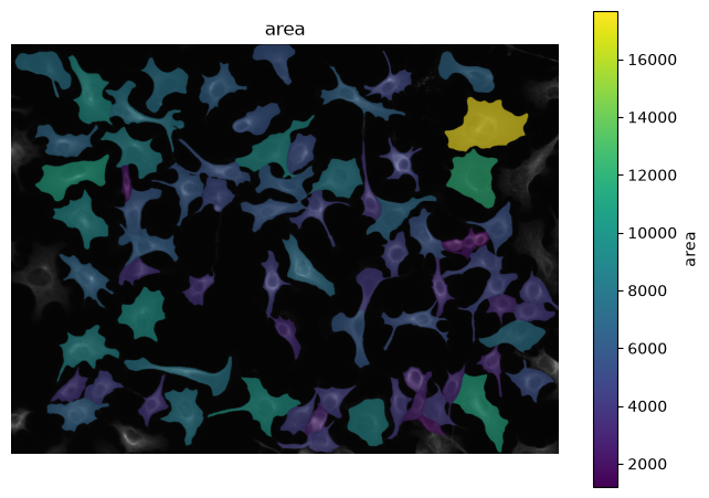
For quality control or exploration it is important to overlay measured quantities on the original image. Here we use the overlay function for that.

overlay_labels(image, labeled_mask, df=df, id_col="cell_id", measurement_col="area")

../../_images/fe93db687940f07aa13ab72f3d89711b095d6454d8b851b41c78ff0d0891c21f.png

Calculate summary statistics and correlation#

Pandas gives us the ability to very effectively compute common summary statistics like mean, median, standard deviation, standard error, etc. on either whole columns or on subsets via aggregation (split by a categorical variable).

# print the average area of all objects
mean_area = df["area"].mean()
print(f"Average area across all objects: {mean_area:.2f} pixels")

Average area across all objects: 5792.17 pixels

# print common statistics for the area feature
print("Area statistics:")
print(f"Mean: {df['area'].mean():.2f} pixels")
print(f"Median: {df['area'].median():.2f} pixels")
print(f"Standard Deviation: {df['area'].std():.2f} pixels")
print(f"Minimum: {df['area'].min()} pixels")
print(f"Maximum: {df['area'].max()} pixels")

Area statistics:
Mean: 5792.17 pixels
Median: 5365.50 pixels
Standard Deviation: 2800.20 pixels
Minimum: 1193.0 pixels
Maximum: 17676.0 pixels

# We can more effectively summarize common features using .describe()
print(df["area"].describe())

count       76.000000
mean      5792.171053
std       2800.202628
min       1193.000000
25%       3985.000000
50%       5365.500000
75%       7424.750000
max      17676.000000
Name: area, dtype: float64

# The .agg() method allows us to specify multiple statiscs at once.
print(df["area"].agg(["mean", "median", "std", "min", "max"]))

mean       5792.171053
median     5365.500000
std        2800.202628
min        1193.000000
max       17676.000000
Name: area, dtype: float64

This is a table of common statistics that can be used either as e.g. df['area'].mean() or df['area'].agg(['mean']).

Function	Description
count	Number of non-NA observations
value_counts	Number of observations per category
sum	Sum of values
mean	Mean of values
median	Arithmetic median of values
min	Minimum
max	Maximum
std	Bessel-corrected sample standard deviation
var	Unbiased variance
sem	Standard error of the mean
skew	Sample skewness (3rd moment)
kurt	Sample kurtosis (4th moment)

We can group (aggregate) the data by categories and calculate summary statistics on each group. This is very useful if we e.g. want to find out if cells that have received a treatment are expressing upregulate a gene or exhibit morphological differences.

We achieve this by using the .groupby() method.

First, let’s group objects by size category (small, medium, large) based on size_category and calculate the average intensity_mean for each size category.

df.groupby(["size_category"])["intensity_mean"].mean()

size_category
small     776.428066
medium    602.484704
large     436.542845
Name: intensity_mean, dtype: float64

We can also group by multiple categories at once. Here we group by size_category and expression and we evaluate the mean circularity.

df.groupby(["size_category", "expression"])["circularity"].mean()

size_category  expression
small          low           0.446059
               high          0.537791
medium         none          0.430270
               low           0.357371
               high          0.265920
large          none          0.470875
               low           0.384508
Name: circularity, dtype: float64

The NaN above indicate that there exist no observation with that combination of categories.

Another very useful statistic to calculate is the correlation between two columns per observation. For this we can use the .corr() method.

# calculate the correlation between area and mean intensity
correlation = df["area"].corr(df["intensity_mean"])
print(f"Correlation between area and mean intensity: {correlation:.2f}")

Correlation between area and mean intensity: -0.62

Combine data from multiple `DataFrames`#

To combine data, e.g. from multiple images or experimental days, it is often necessary to combine dataframes. While this is straightforward, it is important to pay attention to proper ‘book keeping’ because it is easy to lose track of where data comes from and what conditions are associated with it.

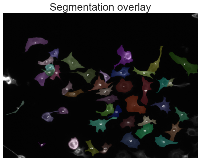
Here we will load the mask and image of the drug treated condition, and measure properties using regionprops_table. We then combine it with our exiting dataframe.

# define the paths to the second image and its corresponding label mask
image_path_2 = Path(
    "../../_static/images/quant/01_measurement_quantification/images/F02_92.TIF"
)
label_path_2 = Path(
    "../../_static/images/quant/01_measurement_quantification/masks/F02_92_cell_labels.tif"
)

# load the second image and label mask
image_2 = tifffile.imread(image_path_2)[1, :, :]
labeled_mask_2 = tifffile.imread(label_path_2)
# remove boundary objects
labeled_mask_2 = skimage.segmentation.clear_border(labeled_mask_2)

# compute region properties for the second image
props_2 = skimage.measure.regionprops_table(
    labeled_mask_2, intensity_image=image_2, properties=properties
)
df_2 = pd.DataFrame(props_2)

print(df_2.head())

---------------------------------------------------------------------------
FileNotFoundError                         Traceback (most recent call last)
Cell In[43], line 10
   "../../_static/images/quant/01_measurement_quantification/masks/F02_92_cell_labels.tif"
)

# load the second image and label mask
---> 10 image_2 = tifffile.imread(image_path_2)[1, :, :]
labeled_mask_2 = tifffile.imread(label_path_2)
# remove boundary objects
labeled_mask_2 = skimage.segmentation.clear_border(labeled_mask_2)

File ~/work/bobiac-book/bobiac-book/.venv/lib/python3.12/site-packages/tifffile/tifffile.py:1256, in imread(files, selection, return_as, aszarr, key, series, kind, level, squeeze, maxworkers, buffersize, mode, name, offset, size, pattern, axesorder, categories, imread, imreadargs, sort, container, chunkshape, chunkdtype, axestiled, ioworkers, chunkmode, fillvalue, zattrs, multiscales, omexml, superres, out, out_inplace, _multifile, _useframes, **kwargs)
       ):
           files = files[0]

       if isinstance(files, str) or not isinstance(files, Sequence):
-> 1256             with TiffFile(
               files,
               mode=mode,
               name=name,

File ~/work/bobiac-book/bobiac-book/.venv/lib/python3.12/site-packages/tifffile/tifffile.py:4554, in TiffFile.__init__(self, file, mode, name, offset, size, omexml, superres, _multifile, _useframes, _root, **is_flags)
               raise ValueError(msg)
           self._omexml = omexml
           self.is_ome = True

-> 4554         fh = FileHandle(file, mode=mode, name=name, offset=offset, size=size)
       self._fh = fh
       self._multifile = True if _multifile is None else bool(_multifile)
       self._files = {fh.name: self}

File ~/work/bobiac-book/bobiac-book/.venv/lib/python3.12/site-packages/tifffile/tifffile.py:12751, in FileHandle.__init__(self, file, mode, name, offset, size)
       self._offset = -1 if offset is None else offset
       self._size = -1 if size is None else size
       self._close = True
       self._lock = contextlib.nullcontext()
> 12751         self.open()
       assert self._fh is not None

File ~/work/bobiac-book/bobiac-book/.venv/lib/python3.12/site-packages/tifffile/tifffile.py:12771, in FileHandle.open(self)
               msg = f'invalid mode {self._mode}'
               raise ValueError(msg)
           self._file = os.path.realpath(self._file)
           self._dir, self._name = os.path.split(self._file)
> 12771             self._fh = open(  # noqa: SIM115
               self._file, self._mode, encoding=None
           )
           self._close = True

FileNotFoundError: [Errno 2] No such file or directory: '/home/runner/work/bobiac-book/bobiac-book/_static/images/quant/01_measurement_quantification/images/F02_92.TIF'

overlay_labels(image_2, labeled_mask_2)

../../_images/56360e384b25d9428baf081d9635307c023b20e73f158e690cd20a36f58c9666.png

(<Figure size 800x800 with 1 Axes>,
 <Axes: title={'center': 'Segmentation overlay'}>)

Now it is absolutely necessary to add a column that identifies where the data came from. In this case we (like above) use the image name as identifier.

# First we add a new column that uniquely identifies each cell in the second dataframe.
# we add 1 to the index to get the correct cell ID corresponding to the label IDs in the labeled mask, which start at 1
df_2["cell_id"] = df_2.index + 1

# add a column to each DataFrame that contains the image ID (e.g., F01_202w1 and F02_92w1)
df_2["image_id"] = image_path_2.stem
print("Second DataFrame with image_id column:")
print(df_2[["image_id"]].head())
print()
print("First DataFrame with image_id column:")
print(df[["image_id"]].head())

Second DataFrame with image_id column:
  image_id
 F02_92
 F02_92
 F02_92
 F02_92
 F02_92

First DataFrame with image_id column:
  image_id
F01_202
F01_202
F01_202
F01_202
F01_202

Now we can use the concat function in pandas to create a merged dataframe from the first and second ones.

# We use pd.concat to concatenate the two DataFrames along the rows (axis=0), which combines all the measurements from both images into a single DataFrame.
# The ignore_index=True argument resets the index of the resulting DataFrame so that it runs from 0 to n-1, where n is the total number of rows in the concatenated DataFrame.
df_combined = pd.concat([df, df_2], ignore_index=True)
print(df_combined)

       area  intensity_mean  intensity_std  intensity_max  intensity_min  \
  5634.0      422.204295     198.333981         1118.0          132.0   
  4728.0      764.301607     523.274140         3509.0          138.0   
  7677.0      279.368894     125.690020         1069.0          118.0   
  6824.0      433.457210     254.054528         1445.0          120.0   
  9638.0      492.971571     267.211757         1934.0          123.0   
..      ...             ...            ...            ...            ...   
7180.0      318.474234     145.186551         1381.0           91.0   
5311.0     2293.158727    1245.594333         4095.0          170.0   
4999.0      327.422284     168.351988         1366.0          100.0   
 918.0      121.674292      27.344323          218.0           72.0   
3597.0      851.481790     780.147753         4095.0          126.0   

      perimeter  intensity_mean_bg_subtracted  intensity_range  cell_id  \
  376.877200                    294.955703            986.0        1   
  516.416306                    637.053015           3371.0        2   
  502.031529                    152.120301            951.0        3   
  444.132034                    306.208617           1325.0        4   
  570.535101                    365.722978           1811.0        5   
..          ...                           ...              ...      ...   
442.132034                           NaN              NaN       39   
278.492424                           NaN              NaN       40   
414.374675                           NaN              NaN       41   
162.752309                           NaN              NaN       42   
309.462987                           NaN              NaN       43   

     intensity_sum  circularity image_id size_category expression condition  \
      2378699.0     0.498456  F01_202        medium        low   control   
      3613618.0     0.222786  F01_202        medium       high   control   
      2144715.0     0.382771  F01_202        medium       none   control   
      2957912.0     0.434735  F01_202        medium        low   control   
      4751260.0     0.372076  F01_202         large        low   control   
..             ...          ...      ...           ...        ...       ...   
          NaN          NaN   F02_92           NaN        NaN       NaN   
          NaN          NaN   F02_92           NaN        NaN       NaN   
          NaN          NaN   F02_92           NaN        NaN       NaN   
          NaN          NaN   F02_92           NaN        NaN       NaN   
          NaN          NaN   F02_92           NaN        NaN       NaN   

    sum_classified circularity_class  
           high               low  
           high               low  
           high               low  
           high               low  
           high               low  
..             ...               ...  
          NaN               NaN  
          NaN               NaN  
          NaN               NaN  
          NaN               NaN  
          NaN               NaN  

[119 rows x 17 columns]

There are lot’s of NaN values in the lower part of the dataframe. Those correspond to entries that we have computed in the first dataframe but not the second. To avoid this, we can use the parameter join and set it to inner. This way only columns that exist in both dataframes will be kept. outer retains all columns from both dataframes as we have seen above.

df_combined = pd.concat([df, df_2], ignore_index=True, join="inner")
print(df_combined)

       area  intensity_mean  intensity_std  intensity_max  intensity_min  \
  5634.0      422.204295     198.333981         1118.0          132.0   
  4728.0      764.301607     523.274140         3509.0          138.0   
  7677.0      279.368894     125.690020         1069.0          118.0   
  6824.0      433.457210     254.054528         1445.0          120.0   
  9638.0      492.971571     267.211757         1934.0          123.0   
..      ...             ...            ...            ...            ...   
7180.0      318.474234     145.186551         1381.0           91.0   
5311.0     2293.158727    1245.594333         4095.0          170.0   
4999.0      327.422284     168.351988         1366.0          100.0   
 918.0      121.674292      27.344323          218.0           72.0   
3597.0      851.481790     780.147753         4095.0          126.0   

      perimeter  cell_id image_id  
  376.877200        1  F01_202  
  516.416306        2  F01_202  
  502.031529        3  F01_202  
  444.132034        4  F01_202  
  570.535101        5  F01_202  
..          ...      ...      ...  
442.132034       39   F02_92  
278.492424       40   F02_92  
414.374675       41   F02_92  
162.752309       42   F02_92  
309.462987       43   F02_92  

[119 rows x 8 columns]

Now we don’t have any NaNs anymore. But we have also lost all the new columns we generated on the first dataframe. It is therefore generally advised to merge dataframes before doing calculations or classifications or to perform them in parallel on all dataframes using e.g. a for loop.

Handle strings in DataFrames#

It is often very handy to manipulate strings in a dataframe column. Especially when files are consistently named, this can save a lot of effort when categorising data.

For example: our images are called F01_202w1 and F02_92w1. Say, F01 would be the well with the control and F02 is the well with a drug. We can use the image_id column to create a new column with those labels.

For that we can use the .str method on the image_id column, which allows us to do string operations like split in bulk.

# Step 0: create a dictionary that maps the well id to the experimental condition
dict_condition = {"F01": "control", "F02": "drug"}

# Step 1: Turn the image_id column into a string-like object
print("1. String-like object\n", df_combined["image_id"].str)

# Step 2: use split on '_' to split each entry into a list of two strings
print("\n2. Split strings\n", df_combined["image_id"].str.split("_"))

# Step 3: Select only the first entry of each list
print("\n3. Select first entry\n", df_combined["image_id"].str.split("_").str[0])

# Step 4: Replace the well id with the experimental condition
print(
    "\n4. Replace:\n",
    df_combined["image_id"].str.split("_").str[0].replace(dict_condition),
)

df_combined["condition"] = (
    df_combined["image_id"].str.split("_").str[0].replace(dict_condition)
)

String-like object
 <pandas.core.strings.accessor.StringMethods object at 0x1289a1030>

Split strings
    [F01, 202]
    [F01, 202]
    [F01, 202]
    [F01, 202]
    [F01, 202]
          ...    
   [F02, 92]
   [F02, 92]
   [F02, 92]
   [F02, 92]
   [F02, 92]
Name: image_id, Length: 119, dtype: object

Select first entry
    F01
    F01
    F01
    F01
    F01
      ... 
  F02
  F02
  F02
  F02
  F02
Name: image_id, Length: 119, dtype: object

Replace:
    control
    control
    control
    control
    control
        ...   
     drug
     drug
     drug
     drug
     drug
Name: image_id, Length: 119, dtype: object

Saving DataFrames as CSV#

A key advantage of the DataFrame is that it can be stored as a CSV (comma separated values) file that can be opened in Excel, Prism, R or any other data analysis software.

For that we simply use the .to_csv method on a DataFrame.

# index=False ensures that the index column of the dataframe is not saved with the rest of the data
df_combined.to_csv("combined_measurements.csv", index=False)

To load a CSV file into a Dataframe, we use the read_csv function.

df_loaded = pd.read_csv("combined_measurements.csv")
print(df_loaded)

       area  intensity_mean  intensity_std  intensity_max  intensity_min  \
  5634.0      422.204295     198.333981         1118.0          132.0   
  4728.0      764.301607     523.274140         3509.0          138.0   
  7677.0      279.368894     125.690020         1069.0          118.0   
  6824.0      433.457210     254.054528         1445.0          120.0   
  9638.0      492.971571     267.211757         1934.0          123.0   
..      ...             ...            ...            ...            ...   
7180.0      318.474234     145.186551         1381.0           91.0   
5311.0     2293.158727    1245.594333         4095.0          170.0   
4999.0      327.422284     168.351988         1366.0          100.0   
 918.0      121.674292      27.344323          218.0           72.0   
3597.0      851.481790     780.147753         4095.0          126.0   

      perimeter  cell_id image_id condition  
  376.877200        1  F01_202   control  
  516.416306        2  F01_202   control  
  502.031529        3  F01_202   control  
  444.132034        4  F01_202   control  
  570.535101        5  F01_202   control  
..          ...      ...      ...       ...  
442.132034       39   F02_92      drug  
278.492424       40   F02_92      drug  
414.374675       41   F02_92      drug  
162.752309       42   F02_92      drug  
309.462987       43   F02_92      drug  

[119 rows x 9 columns]

Concluding remarks on `pandas`#

This is only a brief overview of the capabilities of pandas.

There are several great resources that go deeper. Check out the pandas tutorials or community tutorials.

Success#

Now we have a tidy table that contains all cells of the control and drug treated conditions and their corresponding properties, including area and intensity_mean. This will allow us to make a statement about the effect of the drug and maybe answer our question, which was: Do drug treated cells exhibit changes in F-actin abundance or size?

Plotting results with `seaborn`#

To plot results contained in a DataFrame, we can use the seaborn plotting library which is based on matplotlib and allows for straightforward usage of categorical and numerical data and gives access to standard plots like bar graphs, violin plots, histograms, heatmaps, line plots, regression plots, etc. See the seaborn gallery for inspiration.

import seaborn as sns

# Specifying some figure aesthetics
sns.set_context("poster")
sns.set_style("ticks")

Histogram#

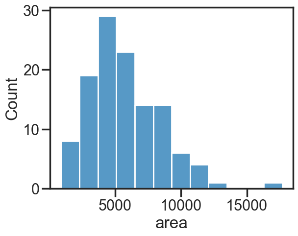
A great tool for looking at distributions of values. Here we use the histplot function. Unlike in matplotlib we do not hand lists or arrays to the x (and y) parameters; instead we specify a DataFrame as data and assign columns as x (and later y).

sns.histplot(data=df_combined, x="area")

<Axes: xlabel='area', ylabel='Count'>

../../_images/8f0d2a3a990656bbdf800bb57d5d7da04c720200884185a67065db2b73d71606.png

Box plot#

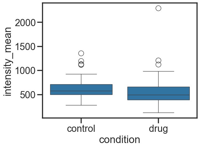
One common way of displaying results is as a box plot. Here we use the boxplot function to create one.

sns.boxplot(data=df_combined, x="condition", y="intensity_mean")

<Axes: xlabel='condition', ylabel='intensity_mean'>

../../_images/81795af9d41367cb0261cb9fa6d536def104cfe7ac1ff938257107cfedd43d6d.png

Violin plot#

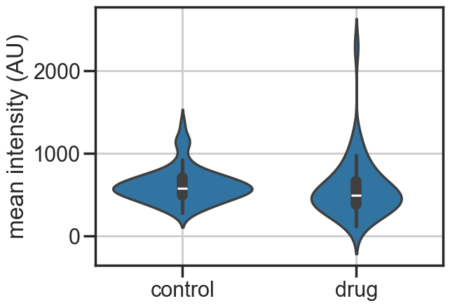
To generate a violin plot we use the violinplot function. Note that the arguments of the plotting function are conserved between violinplot and boxplot. This is the case for most seaborn plotting functions. Moreover, since seaborn is using matplotlib, we can use matplotlib commands to adjust the figure. Here we add a grid and change the axis labels.

sns.violinplot(data=df_combined, x="condition", y="intensity_mean")
plt.grid()  # add grid
plt.xlabel("")  # remove x label
plt.ylabel("mean intensity (AU)")  # overwrite y label

Text(0, 0.5, 'mean intensity (AU)')

../../_images/b981d0b26d9e86e20357d97f7c31eefcc54bed13831f413b9c1d8a50dc112bb3.png

Bar graph#

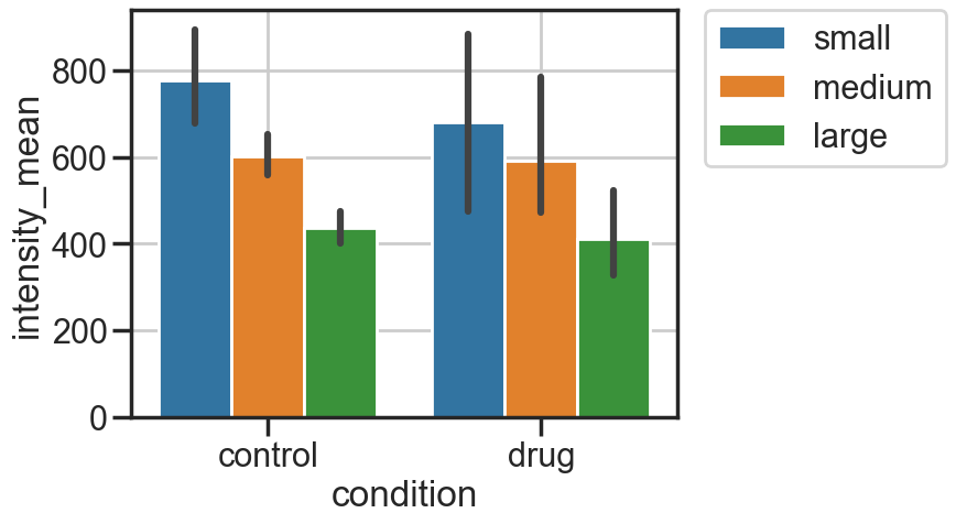
The seaborn function for that is barplot and it follows the same pattern as the two previous plots. Here we demonstrate another very useful function of seaborn plots which is splitting data by a second category.

Say, we would like to explore the difference in expression between the control and drug is driven by higher expression only in small cells. After generating size categories based on their area, we can use the hue parameter to split each condition into several bars. This of course also works for the plots above.

# Create new column that categorises cells as 'small', 'medium' and 'large' as we did before
df_combined["size_category"] = pd.cut(
    df_combined["area"],
    bins=[0, 4000, 8000, np.inf],
    labels=["small", "medium", "large"],
)

sns.barplot(
    data=df_combined,
    x="condition",
    y="intensity_mean",
    hue="size_category",
)
plt.grid()
# move legend outside of the plot
plt.legend(bbox_to_anchor=(1.05, 1), loc=2, borderaxespad=0.0)

<matplotlib.legend.Legend at 0x128d22470>

../../_images/c87a2a202e9ad0c8bd0f87ff0dbf5833d2fe78b169257eac92ac7fb83f7da8fe.png

Scatter plot#

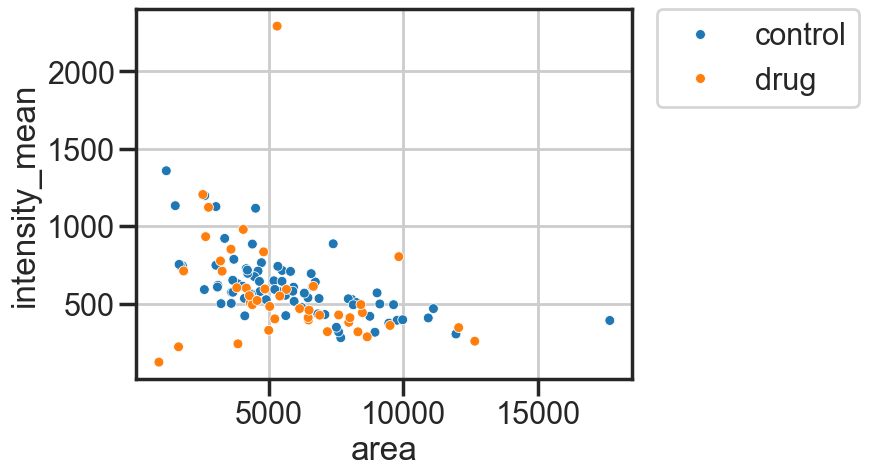
To plot two continuous variables against each other we can use scatterplot.

sns.scatterplot(
    data=df_combined,
    x="area",
    y="intensity_mean",
    hue="condition",
    s=50,  # controls the size of the dots
)
plt.grid()
plt.legend(bbox_to_anchor=(1.05, 1), loc=2, borderaxespad=0.0)

<matplotlib.legend.Legend at 0x128dd86a0>

../../_images/00fe494f21b3fb49989522449a6451a36af622232de66b4ad9897e801e1454ea.png

✍️ Exercise: Plot the results for area changes#

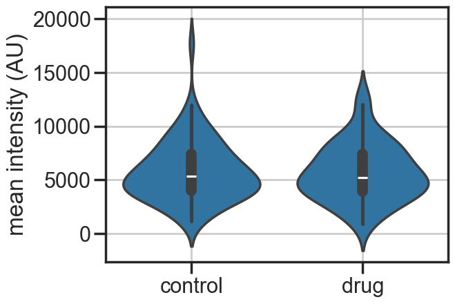
Create a violinplot that shows the differences in cell size between control and drug treatment.
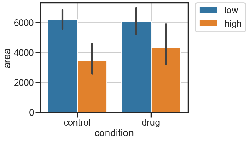
Classify intensity_mean into low and high using the threshold 750 and plot area by condition split by this classification.
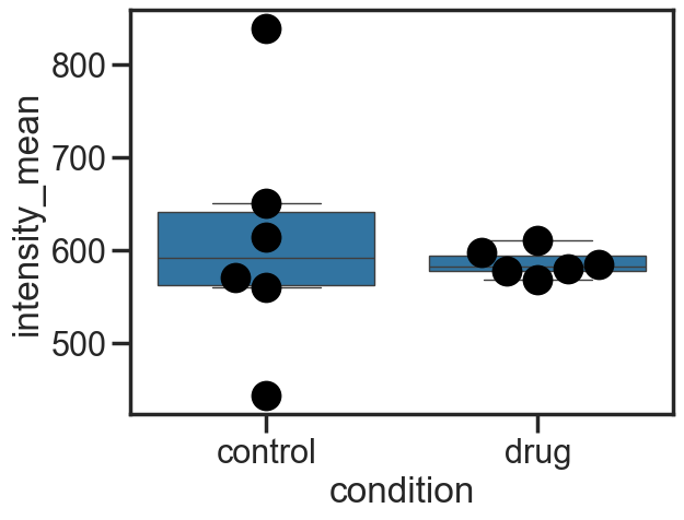
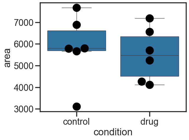
Create swarmplots for area by condition and intensity_mean by condition. Look up swarmplot in the seaborn documentation.

sns.violinplot(data=df_combined, x="condition", y="area")
plt.grid()  # add grid
plt.xlabel("")  # remove x label
plt.ylabel("mean intensity (AU)")  # overwrite y label

Text(0, 0.5, 'mean intensity (AU)')

../../_images/2d76af1beb65bf31ee5243d7fa7bb40be29cd8fc2bee7af97c22e23a2ec56bfe.png

df_combined["expression"] = pd.cut(
    df_combined["intensity_mean"], bins=[0, 750, np.inf], labels=["low", "high"]
)
sns.barplot(
    data=df_combined,
    x="condition",
    y="area",
    hue="expression",
)
plt.grid()
# move legend outside of the plot
plt.legend(bbox_to_anchor=(1.05, 1), loc=2, borderaxespad=0.0)

<matplotlib.legend.Legend at 0x1285b6c80>

../../_images/f7c6ab617fdd29d1442847c958877d98f7fb6ab7909a3d5fd0becfb7bef91d0a.png

Bringing it all together - batch processing#

To process more than a hand full of images, we can automate the measurement process.

properties = [
    "area",
    "intensity_mean",
    "label",
]

image_folder = Path("/Users/max/Desktop/bobiac_data/04_05_06_07_seg_and_spot/")
mask_folder = Path("/Users/max/Desktop/bobiac_data/04_05_06_07_seg_and_spot_labels_and_spots_coords/cells_labels/")

images = sorted(image_folder.glob("*.tif"))
masks = sorted(mask_folder.glob("*.tif"))

list_df = []

for i, image_path in enumerate(images):
    mask_path = masks[i]
    img_name = image_path.stem

    # load the image and label mask
    image = tifffile.imread(image_path)[1, :, :]
    mask = tifffile.imread(mask_path)
    mask = skimage.segmentation.clear_border(mask)  # remove boundary objects

    # compute region properties for the second image
    props = skimage.measure.regionprops_table(
        mask, intensity_image=image, properties=properties
    )
    sdf = pd.DataFrame(props)

    # create additional columns for book keeping
    sdf["image_id"] = img_name

    if img_name[:3] == "F01":
        condition = "control"
    elif img_name[:3] == "F02":
        condition = "drug"
    else:
        condition = "unknown"
    sdf["condition"] = condition

    # add dataframe to a list
    list_df.append(sdf)
# combine all dataframes into one
df_full = pd.concat(list_df)

print(df_full)

      area  intensity_mean  label image_id condition
 5634.0      422.204295      1  F01_202   control
 4728.0      764.301607      2  F01_202   control
 7677.0      279.368894      3  F01_202   control
 6824.0      433.457210      4  F01_202   control
 9638.0      492.971571      5  F01_202   control
..     ...             ...    ...      ...       ...
7180.0      318.474234     43   F02_92      drug
5311.0     2293.158727     44   F02_92      drug
4999.0      327.422284     45   F02_92      drug
 918.0      121.674292     47   F02_92      drug
3597.0      851.481790     48   F02_92      drug

[858 rows x 5 columns]

df_plot = (
    df_full.groupby(["condition", "image_id"])[["area", "intensity_mean"]]
    .mean()
    .reset_index()
)

print(df_plot)

   condition image_id         area  intensity_mean
  control  F01_202  5792.171053      613.218862
  control  F01_204  5795.350000      650.675463
  control  F01_291  6880.835821      442.783777
  control  F01_366  7671.062500      559.852406
  control  F01_508  5659.150943      838.700329
  control  F01_589  3109.155039      569.854286
     drug  F02_110  5249.031250      610.595584
     drug  F02_321  4117.043478      584.439157
     drug  F02_370  7186.200000      596.836724
     drug  F02_696  6556.510204      579.760313
    drug  F02_776  4259.308642      568.131303
    drug   F02_92  5698.465116      576.990540

sns.boxplot(
    data=df_plot,
    x="condition",
    y="intensity_mean",
)

sns.swarmplot(data=df_plot, x="condition", y="intensity_mean", c="k", s=20)

<Axes: xlabel='condition', ylabel='intensity_mean'>

../../_images/82f8362e547e701b75d6d75c4e8ab1b51b9af5e2978cbe5183ab0cc85b18e07a.png

sns.boxplot(
    data=df_plot,
    x="condition",
    y="area",
)

sns.swarmplot(data=df_plot, x="condition", y="area", c="k", s=20)

<Axes: xlabel='condition', ylabel='area'>

../../_images/b6df7e146a0a6e02d2a6fc1a7756013118838acf2bfe4238cefc87530c97b873.png

Conclusion#

We successfully measured properties of cells and compared them with each other. In the following notebooks we will explore two common types of analysis: nested measurements and time series data. Now that we know regionprops_table, pandas and seaborn this will be relatively straightforward.