Cellpose in Python

Cellpose in Python#

# /// script
# requires-python = ">=3.12"
# dependencies = [
#     "matplotlib",
#     "cellpose",
#     "tqdm",
#     "ndv[jupyter,pygfx]",
#     "jupyter-rfb<=0.5.4",
# ]
# ///

Overview#

Website | GitHub | Paper | Cellpose Documentation | Cellpose API

In this section, we’ll learn how to use Cellpose, a powerful deep learning tool for cell segmentation, works on a wide variety of microscopy images and doesn’t require retraining for many common use cases.

In this notebook, we’ll see how to run Cellpose on single images or on a folder of images, and how to visualize and save the results.

The images we will use for this section can be downloaded from the Segmentation and Spot Detection Dataset.

NOTE: Windows users, if you encounter an error in ndv similar to:

Failed to load model class 'VBoxModel' from module '@jupyter-widgets/controls' ChunkLoadError at Object.j...

this is usually caused by the default uv cache path being too long. Point uv's cache to a shorter location by running the following in your PowerShell terminal before launching Jupyter, then restart the notebook kernel:

$env:UV_CACHE_DIR = "C:\uvc"

This only affects the current terminal session. To make it permanent for all future sessions (so you don't have to set it every time), run the following once, then close and reopen PowerShell for the change to take effect:

setx UV_CACHE_DIR "C:\uvc"

💡 Tip: Cellpose runs significantly faster on a GPU. It supports both NVIDIA GPUs (CUDA) and Apple Silicon (MPS). If you don't have either, we recommend running this notebook on Google Colab for faster performance.

NVIDIA GPU (CUDA - Windows/Linux)

In order to use Cellpose in this notebook with an NVIDIA GPU:

you need to have the NVIDIA drivers installed on your system.
you can run nvidia-smi in the terminal to check your CUDA version (shown in the top-right of the output, e.g. CUDA Version: 13.0.0).
update the # /// script block at the top of this notebook to install the appropriate version of PyTorch with CUDA support (replace cu130 with your CUDA version):

    # /// script
    # requires-python = ">=3.12"
    # dependencies = [
    #     "matplotlib",
    #     "cellpose",
    #     "tqdm",
    #     "ndv[jupyter,pygfx]",
    #     "jupyter-rfb<=0.5.4",
    #     "torch",
    #     "torchvision",
    # ]
    #
    # [tool.uv.sources]
    # torch = { index = "pytorch-cu130" }
    # torchvision = { index = "pytorch-cu130" }
    #
    # [[tool.uv.index]]
    # name = "pytorch-cu130"
    # url = "https://download.pytorch.org/whl/cu130"
    # explicit = true
    # ///

re-run the notebook using uvx juv run.

Import Libraries#

from pathlib import Path

import matplotlib.pyplot as plt
import ndv
import numpy as np
from cellpose import core, io, models, plot
from cellpose.models import MODEL_DIR
from tqdm import tqdm

Setup#

io.logger_setup()  # to get printing of progress

use_gpu = core.use_gpu()
print("GPU available:", use_gpu)

creating new log file
[GUI INFO] : WRITING LOG OUTPUT TO /home/runner/.cellpose/run.log

cellpose version: 	4.2.1.1 
platform:       	linux 
python version: 	3.12.3 
torch version:  	2.12.1+cu130
2026-07-08 01:28:24,940 [io INFO] WRITING LOG OUTPUT TO /home/runner/.cellpose/run.log

2026-07-08 01:28:24,941 [io INFO] 
cellpose version: 	4.2.1.1 
platform:       	linux 
python version: 	3.12.3 
torch version:  	2.12.1+cu130

2026-07-08 01:28:24,942 [core INFO] Neither TORCH CUDA nor MPS version not installed/working.

GPU available: False

Run Cellpose on a Single Image#

In this section, we’ll apply Cellpose to a single image and visualize the segmentation result.

Load the Image#

To load the image, we can use the imread method from the Cellpose io module (or the tifffile library if you add it to the dependencies).

image_path = "../../../_static/images/cellpose/cell_cellpose.tif"
image = io.imread(image_path)  # or image = tifffile.imread(image_path)

Let’s inspect the image shape. How many channels do we have?

print(image.shape)

(5, 1040, 1392)

We can use the imshow method from the ndv library (or from the matplotlib.pyplot library) to visualize the image.

💡 Note: Since this is a multi-channel image, if using matplotlib, you will need to specify which channel to visualize (e.g. plt.imshow(image[0]) for the first channel).

ndv.imshow(
    image,
    channel_mode="composite",
    luts={
        0: {"cmap": "cyan"},
        1: {"cmap": "magenta"},
        2: {"cmap": "green"},
        3: {"cmap": "yellow"},
        4: {"cmap": "gray"},
    },
)

snapshot

Initialize the Model#

To initialize Cellpose model we can use the models.CellposeModel() class.

There are other parameters we can set when initializing the model, here we will only use pretrained_model to specify which pretrained model to use and gpu to specify whether to use GPU (if available) for faster inference.

Currently, the available pretrained models are:

cpsam: this is the original CellposeSAM model released in April 2025 using the SAM-ViTL backbone (default model)
cpsam_v2: this is the CellposeSAM model released in June 2026 using the SAM-ViTL backbone, it includes a fix in the training for low contrast regions
cpdino: this is the CellposeDINO model released in June 2026 using the DINOv3-ViTL backbone
cpdino-vitb: this is the CellposeDINO model released in June 2026 using the DINOv3-ViTB backbone (smaller model)

Note: Only the default cpsam model is downloaded automatically the first time you run this notebook (this may take a while). The other models (cpsam_v2, cpdino, cpdino-vitb) must be downloaded manually, see below.

Downloading the Other Pretrained Models#

These models are hosted on the Cellpose-SAM Hugging Face repository. We need to download the model and place it in the ~/.cellpose/models directory (the MODEL_DIR variable from the cellpose.models module).

from cellpose.utils import download_url_to_file

model_name = "cpsam_v2"  # or "cpdino" / "cpdino-vitb"

MODEL_DIR.mkdir(parents=True, exist_ok=True)
model_path = MODEL_DIR / model_name
if not model_path.exists():
    url = f"https://huggingface.co/mouseland/cellpose-sam/resolve/main/{model_name}"
    download_url_to_file(url, str(model_path))

Now we can initialize the model with the different pretrained models by setting the pretrained_model parameter.

model_path = str(MODEL_DIR / "cpsam_v2")  # or "cpdino" / "cpdino-vitb" or "cpsam"
model = models.CellposeModel(pretrained_model=model_path, gpu=use_gpu)

Run Cellpose#

After initializing the model, we can run it on the image using the model.eval() method (see dropdown below for parameters details).

We want to run cellpose only on the nuclei and cytoplasm channels (the first two) and not on the spots channels. Therefore, we should pass to the model.eval() method only the first two channels of the image (i.e. image[:2]).

Cellpose model.eval() Parameters

model.eval(
    x,
    channel_axis=None,
    normalize=True,
    invert=False,
    diameter=None,
    flow_threshold=0.4,
    cellprob_threshold=0.0,
    min_size=15,
    max_size_fraction=0.4,
    niter=None,
    compute_masks=True,
    batch_size=8,
    resample=True,
    bsize=256,
    tile_overlap=0.1,
    augment=False,
    do_3D=False,
    z_axis=None,
    anisotropy=None,
    flow3D_smooth=0,
    stitch_threshold=0.0,
)

Input

Parameter	Type	Default	Description
`x`	`np.ndarray \| list[np.ndarray]`	—	A single image or list of images (2D/3D/4D). For `cpsam`, up to 3 channels are used.
`channel_axis`	`int \| None`	`None`	Which axis of `x` is the channel axis. If `None`, Cellpose auto-detects it.

Preprocessing

Parameter	Type	Default	Description
`normalize`	`bool \| dict`	`True`	Normalize intensities to 0–1 using 1st/99th percentile. Pass `False` to skip, or a dict for fine-grained control (see below).
`invert`	`bool`	`False`	Invert pixel intensities before running the network. Useful for brightfield images where cells are dark on a bright background.
`diameter`	`float \| None`	`None`	Expected cell diameter in pixels. Used to rescale the image so cells appear ~30 px wide to the model. If `None`, no rescaling is applied.

When passing normalize as a dict, all keys are optional and can be combined:

# Tile-based normalization: useful when illumination is uneven across the image.
normalize = {"tile_norm_blocksize": 100}

# Fixed intensity range: skip percentile computation and clamp to known values.
normalize = {"lowhigh": [200, 4000]}

# Custom percentiles instead of the default 1st/99th.
normalize = {"percentile": [5, 95]}

# Sharpen before segmenting (value ≈ 1/4 to 1/8 of cell diameter in px).
normalize = {"sharpen": 5}

# Keys can be combined:
normalize = {"tile_norm_blocksize": 100, "percentile": [2, 98]}

Segmentation quality

Parameter	Type	Default	Description
`flow_threshold`	`float`	`0.4`	Maximum allowed flow error for a mask to be kept. Increase to recover more masks (or set to `0.0` to keep all); decrease to discard ill-shaped masks. Not used in 3D.
`cellprob_threshold`	`float`	`0.0`	Minimum cell probability for a pixel to be included in a mask. Decrease to find more/larger masks; increase to suppress dim or spurious detections.
`min_size`	`int`	`15`	Minimum mask area in pixels. Smaller objects are discarded.
`max_size_fraction`	`float`	`0.4`	Masks larger than this fraction of the total image area are removed.
`niter`	`int \| None`	`None`	Number of iterations for the flow integration step. If `None`, set automatically proportional to `diameter`.
`compute_masks`	`bool`	`True`	If `False`, skips flow integration and returns empty masks (useful to get flows/styles only).

Performance

Parameter	Type	Default	Description
`batch_size`	`int`	`8`	Number of image tiles (the image is split into tiles before being processed, see `bsize` below) sent to the GPU together in a single forward pass. Increase for faster throughput (uses more GPU memory); decrease if you hit out-of-memory errors.
`resample`	`bool`	`True`	After the network runs on rescaled tiles, upsample the flow fields back to the original image resolution before tracing cell boundaries. Gives sharper, more precise outlines — especially when `diameter` causes strong downscaling. Disable to speed up processing at the cost of boundary accuracy.
`bsize`	`int`	`256`	Size of each tile in pixels (`bsize × bsize`). For the SAM-based models (`cpsam`, `cpsam_v2`) the positional embeddings are fixed for 256×256 tiles at model-creation time, so changing `bsize` raises a shape-mismatch error (leave at the default). For the DINO-based models (`cpdino`, `cpdino-vitb`) the default is 384 and `bsize` can be increased or decreased.
`tile_overlap`	`float`	`0.1`	Each tile overlaps its neighbors by this fraction. Overlapping regions are averaged, which smooths discontinuities at tile edges. Increase if you see artifacts along grid lines (e.g. for very large cells that span multiple tiles).
`augment`	`bool`	`False`	Run each tile also with horizontal and vertical flips, then average the results. Slightly more robust at tile boundaries but roughly doubles computation time.

3D segmentation

Parameter	Type	Default	Description
`do_3D`	`bool`	`False`	Set to `True` to run full 3D segmentation on a Z-stack.
`z_axis`	`int \| None`	`None`	Which axis is the Z axis (for 3D images). If `None`, auto-detected.
`anisotropy`	`float \| None`	`None`	Ratio of the Z pixel size to the XY pixel size (`Z_pixel_size / XY_pixel_size`). Used to rescale the Z axis so voxels appear isotropic to the model. For example, if your Z step is 2 µm and your XY pixel size is 0.5 µm, set `anisotropy=4.0`. If `None`, voxels are assumed to be isotropic.
`flow3D_smooth`	`float \| list[float]`	`0`	Smooth 3D flows with a Gaussian filter of this stddev. Helps reduce Z-fragmentation and ring artifacts. Can be a list `[z, y, x]` for axis-independent smoothing.
`stitch_threshold`	`float`	`0.0`	If `> 0` and `do_3D=False`, stitch 2D masks across Z slices into a 3D volume.

Returns

Output	Type	Description
`masks`	`np.ndarray \| list[np.ndarray]`	2D label array (or list of them). `0` = background; `1, 2, …` = individual cell IDs.
`flows`	`list`	List of flow outputs per image: `flows[0]` = RGB flow visualization; `flows[1]` = XY flow vectors; `flows[2]` = cell probability map.
`styles`	`np.ndarray`	Style vectors (legacy, all zeros for all models, retained for compatibility with CP3).

cp_image = image[:2]
masks, flows, styles = model.eval(cp_image)

Display the Results#

To display the results, we can use the show_segmentation method from the Cellpose plot module that will show the original image, predicted masks, outlines, and flow fields in a single figure (alternatively, you can use other libraries like ndv or matplotlib to directly visualize the outputs).

fig = plt.figure(figsize=(12, 5))
plot.show_segmentation(fig, cp_image, masks, flows[0])
plt.tight_layout()
# Optional if you want to also save the figure
# plt.savefig(f"path/to/output/{Path(image_path).stem}_cp_output.png")
plt.show()

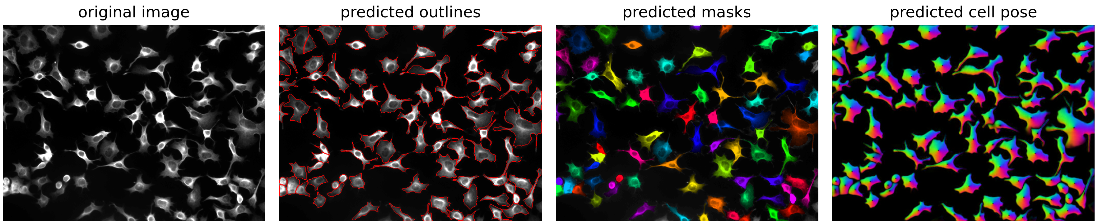
To save the labelled masks as a .tif file, you can use the Cellpose imsave method from the io module (or e.g. the tifffile library if you add it to the dependencies):

output_path = f"path/to/output/{Path(image_path).stem}_labels.tif"
io.imsave(output_path, masks)  # or tifffile.imwrite(output_path, masks)

To override the defaults, pass any parameter explicitly to model.eval() (see hidden cell above). For example, to adjust the segmentation quality parameters:

masks, flows, styles = model.eval(
    cp_image,
    flow_threshold=0.2,
    cellprob_threshold=0.8,
    min_size=800,
)

Run Cellpose on a Folder of Images#

Now that we’ve seen how to run Cellpose on a single image, let’s scale up and apply it to a folder of images. This is useful when you have an entire experiment or dataset that you want to segment automatically.

The simplest way to do this is to just loop through the images in the folder and run model.eval() on each one. During each iteration, we can save the predicted masks to an output folder using the imsave method from the Cellpose io module (or the tifffile library if you add it to the dependencies).

# Path to the folder containing the images to segment
folder_path = Path("data/04_segmentation_cellpose")

# Create a subfolder to save the cell segmentation results
labels_folder = folder_path / "cell_labels"
labels_folder.mkdir(exist_ok=True)

# Get the sorted list of all .tif images in the folder
images_path = sorted(folder_path.glob("*.tif"))

# Initialize the model once before the loop
model_path = str(MODEL_DIR / "cpsam_v2")  # or "cpdino" / "cpdino-vitb" or "cpsam"
model = models.CellposeModel(pretrained_model=model_path, gpu=use_gpu)

# Run Cellpose on each image one by one
# NOTE: tqdm is used to show a progress bar, but you can remove it if you don't want it
for image_path in tqdm(images_path, desc="Processing images"):
    # Load the image
    image = io.imread(image_path)
    # Select only the first two channels for Cellpose
    cp_image = image[:2]
    # Run Cellpose on the image
    masks, flows, styles = model.eval(cp_image)
    # Save the segmentation results as a TIFF file
    output_path = labels_folder / f"{image_path.stem}_labels.tif"
    io.imsave(output_path, masks)  # or tifffile.imwrite(output_path, masks)

Bonus 1: Cellpose 3D Segmentation#

Running a 3D segmentation on a z-stack is not very different than running it on a 2D image, you just need to set do_3D=True and specify the z_axis and, if needed, anisotropy (see the model.eval() parameter dropdown above and the 3D Cellpose documentation for more details).

The images we will use for this section can be downloaded from the Cellpose 3D Dataset.

Load the 3D Image#

image_path = "../../../_static/images/cellpose/cell_cellpose_3d.tif"
image = io.imread(image_path)  # or image = tifffile.imread(image_path)

print(image.shape)

For 3D segmentation, it is important to know the scale of the image in the XY and Z dimensions (e.g. from the metadata) so that we can set the anisotropy parameter correctly.

For this sample image, we have: XY pixel size = 0.202 µm Z step size = 0.5 µm

scale_x = 0.202
scale_y = 0.202
scale_z = 0.5
anisotropy = scale_z / scale_x
print("Anisotropy:", anisotropy)

Visualize the 3D Image#

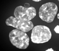
We can visualize the max intensity projection of the stack using matplotlib.

💡 Note: If running the notebook locally (not on Google Colab), we can visualize the image using ndv. We can pass the scales parameter to set the scale for each axis (Z, Y, X) and correctly visualize the volume.

import ndv
# the shape of the image is (Z, Y, X) so we need to pass the scales in the same order
ndv.imshow(image, scales={0: scale_z, 1: scale_y, 2: scale_x})

# Create the max intensity projection image
max_p = np.max(image, axis=0)

# Visualize the max intensity projection image
plt.imshow(max_p, cmap="gray")
plt.axis("off")
plt.tight_layout()
plt.show()

# We can also visualise the reslice of the image acros the XZ dimension
plt.imshow(image[:, 110, :], cmap="gray")
plt.axis("off")
plt.tight_layout()
plt.show()

Initialize the model#

model_path = str(MODEL_DIR / "cpsam_v2")  # or "cpdino" / "cpdino-vitb" or "cpsam"
model = models.CellposeModel(pretrained_model=model_path, gpu=use_gpu)

Run Cellpose in 3D#

masks, flows, styles = model.eval(
    image, do_3D=True, z_axis=0, anisotropy=anisotropy, flow3D_smooth=1
)

Visualize the results#

We can visualize the results using the show_segmentation method from the Cellpose plot module (one slice at a time).

💡 Note: If running the notebook locally (not on Google Colab), we can visualize the result labeled image using ndv. We can pass the scales parameter to set the scale for each axis (Z, Y, X) and correctly visualize the volume.

import ndv
# the shape of the image is (Z, Y, X) so we need to pass the scales in the same order
ndv.imshow(masks, scales={0: scale_z, 1: scale_y, 2: scale_x})

z = 21  # pick a slice
fig = plt.figure(figsize=(12, 5))
plot.show_segmentation(fig, image[z], masks[z], flows[0][z])
plt.tight_layout()
plt.show()

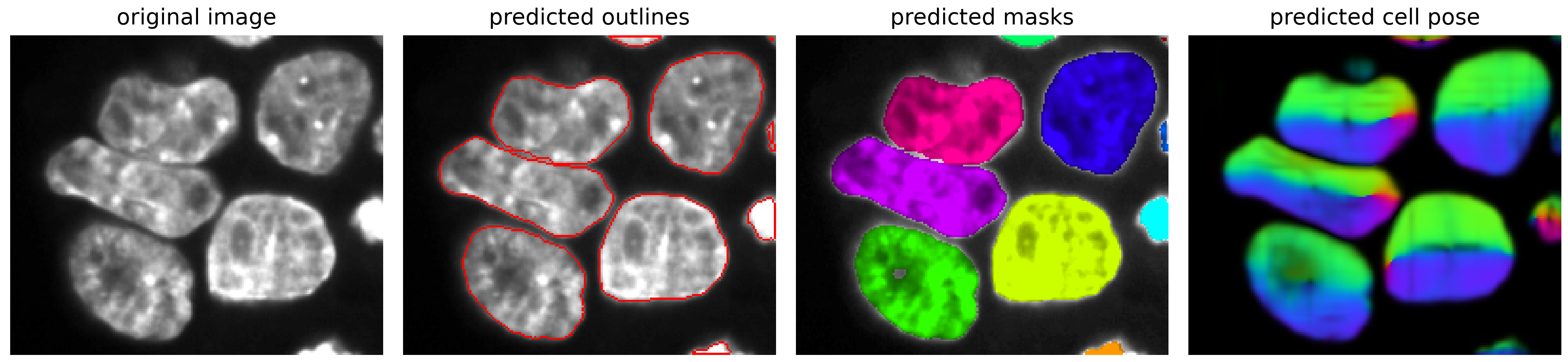
Save the results#

To save the labelled masks as a .tif file, you can use the Cellpose imsave method from the io module (or e.g. the tifffile library if you add it to the dependencies):

output_path = f"path/to/output/{Path(image_path).stem}_3d_labels.tif"
io.imsave(output_path, masks)  # or tifffile.imwrite(output_path, masks)

Info 1: Timelapse Batch Processing#

When working with a timelapse, you cannot pass the raw stack array directly to model.eval(), Cellpose has no concept of timepoints and would misinterpret the time axis as channels or a z-stack.

The solution is to convert the stack into a list of frames using list(stack), which slices along axis 0. The result depends on your axis order:

# TCYX — axis 0 is time → list gives T frames of shape (C, Y, X)
stack.shape  # (10, 2, 512, 512)
list(stack)  # → [frame_0, ..., frame_9], each (2, 512, 512)

So we can pass the list of frames directly to model.eval():

frame_masks, frame_flows, frame_styles = model.eval(list(stack))

frame_masks will be a list of 2D label arrays, one per timepoint.

If the time axis is not the first one (e.g. CTYX), you need to transpose the stack first to get it into TCYX order before converting to a list:

# CTYX — axis 0 is channel → wrong, need to transpose first
stack.shape  # (2, 10, 512, 512)
stack = stack.transpose(1, 0, 2, 3)  # CTYX → TCYX, then list(stack) works

Now that the stack is in TCYX order, you can pass it as a list to model.eval() and Cellpose will process each frame independently, returning one mask per frame.

frame_masks, frame_flows, frame_styles = model.eval(list(stack))

data = Path("/Users/fdrgsp/Desktop/bobiac_exercises_oscillations/F01_1615_tcyx.tif")
data = io.imread(data)  # or image = tifffile.imread(image_path)
t0 = data[0]

frame_masks, frame_flows, frame_styles = model.eval(t0[0])
tiff_output_path = "/Users/fdrgsp/Desktop/bobiac_exercises_oscillations/F01_1615_tcyx_nuclei_labels.tif"
io.imsave(tiff_output_path, frame_masks)

frame_masks, frame_flows, frame_styles = model.eval(t0[[0, 1]])
tiff_output_path = "/Users/fdrgsp/Desktop/bobiac_exercises_oscillations/F01_1615_tcyx_cell_labels.tif"
io.imsave(tiff_output_path, frame_masks)

Info 2: GPU Optimization with `batch_size`#

The simple loop above uses the default batch_size=8. This controls how many 256×256 tiles are sent to the GPU per forward pass.

For each image, Cellpose splits it into overlapping tiles (10% overlap by default) and runs the network on them in groups of batch_size. Increasing batch_size reduces the number of GPU passes per image, which can be faster, at the cost of more GPU memory.

💡 Note: batch_size counts tiles, not images. Even when you loop and pass one image at a time (as above), the knob still matters because a single image is split into many tiles. Note also that passing a list of separate 2D images to model.eval() does not run them in parallel on the GPU: internally Cellpose simply loops over the list one image at a time, so the GPU behaviour is identical to the manual for loop.

How many tiles does an image produce?

The image is divided into 256×256 tiles with a 10% overlap between neighbors, and tiles are added to ensure the edges are fully covered. The total number of tiles grows with image size.

For example, a 1392×1040 image produces 5×7 = 35 tiles:

`batch_size`	GPU passes (35 tiles)
8 (default)	5
16	3
32	2
64	1

Since this image only ever produces 35 tiles, raising batch_size above 35 has no effect for it: the extra capacity simply goes unused.

⚠️ The speedup depends on your GPU. Fewer GPU passes is not automatically faster, it depends on the hardware. On NVIDIA (CUDA) GPUs, packing more tiles into each pass typically reduces wall-clock time. On Apple Silicon (MPS), however, we measured essentially no difference between batch_size=8 and 64 on the image above (~16 s either way): the tiles are not processed any faster in larger batches. On such hardware there is no speed reason to raise batch_size, the only reason to change it is to lower it (using less GPU memory) if you run into out-of-memory errors. It is worth benchmarking on your own machine before tuning this parameter.

On a CUDA GPU, a common strategy is to increase batch_size until you hit out-of-memory errors, then back off one step.

Note: The tile overlap can be adjusted using the tile_overlap parameters in model.eval(). The default is 0.1 (10%) overlap which is the value used during training, so it is recommended to keep it as default unless you have specific reasons to change it.

# Path to the folder containing the images to segment
folder_path = Path("data/04_segmentation_cellpose")

# Create a subfolder to save the cell segmentation results
labels_folder = folder_path / "cell_labels"
labels_folder.mkdir(exist_ok=True)

# Get the sorted list of all .tif images in the folder
images_path = sorted(folder_path.glob("*.tif"))

# Increase batch_size to reduce GPU passes per image (uses more GPU memory)
batch_size = 8  # each pass sends batch_size tiles of 256×256 to the GPU
for image_path in tqdm(images_path, desc="Processing images"):
    image = io.imread(image_path)
    masks, flows, styles = model.eval(image, batch_size=batch_size)
    output_path = labels_folder / f"{image_path.stem}_labels.tif"
    io.imsave(output_path, masks)