
From Ilastik Masks to Labels#
 Open in Colab
# /// script
# requires-python = ">=3.12"
# dependencies = [
#     "matplotlib",
#     "ndv[jupyter,pygfx]",
#     "jupyter-rfb<=0.5.4",
#     "numpy",
#     "scikit-image",
#     "scipy",
#     "tifffile",
#     "imagecodecs",
# ]
# ///
Description#
This notebook demonstrates how to convert the semantic segmentation generated by Ilastik (Simple Segmentation) into instance segmentation.
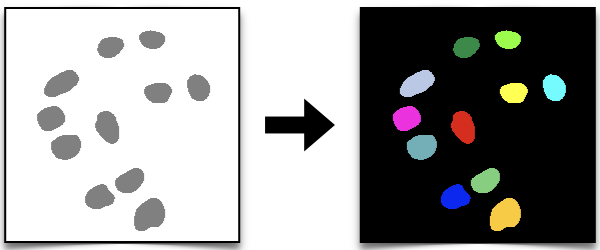
We first explore the type of data that we generated with Ilastik in the previous section (Ilastik for Pixel Classification) and we then use them to generate labels, which can be used for instance segmentation (as we did in the classical segmentation methods) section.
Note: This approach works well for roundish object types, such as nuclei, or any object type that is well separated in the semantic segmentation. For more complex or different object types, a different approach than the distance transform and watershed we use here might be needed.
As mentioned in the previous Pixel Classification With Ilastik section, you could export the Probabilities from the Prediction Export step instead of the Simple Segmentation. If you do so, in the Object Classification section you can load the probability maps and use the Thresholding and Size Filter applet to go directly from probability maps to an instance segmentation.
ndv similar to:
Failed to load model class 'VBoxModel' from module '@jupyter-widgets/controls' ChunkLoadError at Object.j...uv cache path being too long. Point uv's cache to a shorter location by running the following in your PowerShell terminal before launching Jupyter, then restart the notebook kernel:
$env:UV_CACHE_DIR = "C:\uvc"setx UV_CACHE_DIR "C:\uvc"Import libraries#
from pathlib import Path

import matplotlib.pyplot as plt
import ndv
import numpy as np
import tifffile
from scipy import ndimage
from skimage import color, feature, measure, segmentation
Explore the Data#
Let’s first load one of the _Simple Segmentation.tif files and explore the data that we generated with Ilastik. We want to know the type of data that we have before we can convert it to labels (instance segmentation).
Choose one of the _Simple Segmentation.tif file paths and store it in a variable called seg_path.
# set the path to one of the *_Simple Segmentation.tif files
seg_path = "../../../_static/images/ilastik/ilastik_Simple Segmentation.tif"
We can use the tifffile library to read the tif file.
# Load a mask
seg = tifffile.imread(seg_path)
What is the data type?
print(seg.dtype)
print(type(seg))
uint8
<class 'numpy.ndarray'>
We can now use the ndv (or matplotlib) library to display the data and explore the pixel values.
What are the values? Is this a [0 1] binary mask?
# show the mask image
ndv.imshow(seg)

By exploring the results we can notice that all the pixels within the nuclei regions have a value of 1, while the background has a value of 2.
This is because Ilastik assigns numbers to classes starting from 1, based on the number and the order of the classes defined during the training phase. In our case, we defined two classes: the first class corresponds to the nuclei, and the second class corresponds to the background. As a result, the nuclei are labeled with the value 1 and the background with the value 2.
Remember that in order to generate labels from the data, we need binary masks with pixel values of 0 for the background and 1 for our object of interest, the nuclei.
How can we convert them to binary?
Data to Binary Masks#
# Convert to a binary mask
# The nuclei pixels have all value 1, the seg image is a numpy array.
# We can create a new bunary mask by keeping only the pixels with value 1.
binary_mask = seg == 1
If we explore the binary masks with ndv, we can now see that the background has a value of 0 and the nuclei have a value of 1.
# ndv does not like boolean arrays -> convert to uint8 (from False/True to 0/1)
# print(binary_mask.dtype)
ndv.imshow(binary_mask.astype(np.uint8))
Binary Masks to Labels#
Now that we have the binary mask, we can convert it to labels (instance segmentation) as we did in the classic segmentastion methods section.
# compute the distance transform
distance = ndimage.distance_transform_edt(binary_mask)
# find local maxima in the distance transform
local_maxima_coords = feature.peak_local_max(
    distance, footprint=np.ones((25, 25)), min_distance=10
)
# create a binary image from the local maxima coordinates
local_maxima = np.zeros_like(binary_mask, dtype=bool)
local_maxima[tuple(local_maxima_coords.T)] = True
# use the local maxima to create seeds for the watershed algorithm
seeds = measure.label(local_maxima)
# apply the watershed algorithm to segment the image and get labels
labels = segmentation.watershed(-distance, seeds, mask=binary_mask)
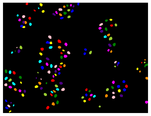
We can now plot the labels and check the results using scikit-image’s label2rgb function.
img = color.label2rgb(labels, bg_label=0)
plt.imshow(img)
plt.axis("off")
plt.show()
We can also save the labels as a tif file using the tifffile library.
NOTE: The dtype of a labeled image is important because it will determine the maximum number of labels that can be stored in the image. In a labeled image, each object is assigned a unique numerical label, and the dtype determines the range of numbers that can be used for labeling (e.g. uint8 -> max 255 objects).
By default, labels generated with the skimage.measure.label function are of type uint32, which is also one of the types that Ilastik requires when we will explore the Object Classification workflow. Therefore, we will use uint32 as the dtype when saving the labels image.
tifffile.imwrite("ilastik_Simple Segmentation_labels.tif", labels.astype("uint32"))
Batch Processing#
Now we understand how to deal with the Simple Segmentation data from Ilastik. In order to obtain instance segmentation from all the _Simple Segmentation.tif files we generated, we can modify the for loop code we wrote at the end of the classic segmentation methods section by adding the line of code where we select only pixels with a value of 1. Doing so will only consider the nuclei in the labelled images.
✍️ Exercise: Batch Masks to Labels#
Write a script that will convert all of the _Simple Segmentation.tif images generated by Ilastik into labeled images (instance segmentation) and save them as tif files.
# make a function to create labels from a _Simple Segmentation.tif file
def ilastik_seg_to_labels(seg_image: np.ndarray, object_index: int) -> np.ndarray:
    """Convert an ilastik simpole segmentation image to labeled image.

    Parameters
    ----------
    seg_image : np.ndarray
        The input segmentation image generated by ilastik.
    object_index : int
        The index of the object to segment (e.g. 1 if your objects have value 1).
    """
    # convert to a binary mask
    binary_mask = seg_image == object_index
    # compute the distance transform
    distance = ndimage.distance_transform_edt(binary_mask)
    # find local maxima in the distance transform
    local_maxima_coords = feature.peak_local_max(
        distance, footprint=np.ones((25, 25)), min_distance=10
    )
    # create a binary image from the local maxima coordinates
    local_maxima = np.zeros_like(binary_mask, dtype=bool)
    local_maxima[tuple(local_maxima_coords.T)] = True
    # use the local maxima to create seeds for the watershed algorithm
    seeds = measure.label(local_maxima)
    # apply the watershed algorithm to segment the image and get labels
    return segmentation.watershed(-distance, seeds, mask=binary_mask)


# set the input directory to the path of the _Simple Segmentation.tif files
input_dir = Path("my_input_directory")
# set the output directory to save the labels
output_dir = Path("my_output_directory")

for seg_file in input_dir.glob("*_Simple Segmentation.tif"):
    print(f"Processing {seg_file.name}...")
    seg_image = tifffile.imread(seg_file)
    labels = ilastik_seg_to_labels(seg_image, object_index=1)
    output_file = output_dir / f"{seg_file.stem}_labels.tif"
    tifffile.imwrite(output_file, labels.astype("uint32"))