Classical Segmentation

Classical Segmentation#

# /// script
# requires-python = ">=3.12"
# dependencies = [
#     "matplotlib",
#     "ndv[jupyter,pygfx]",
#     "jupyter-rfb<=0.5.4",
#     "numpy",
#     "scikit-image",
#     "scipy",
#     "tifffile",
# ]
# ///

Overview#

This notebook covers the following steps in building a classic segmentation pipeline:

Step	Concept	Why it matters
0	Setup	Import dependencies
1	Loading an Image	Open tif image and display it
2	Filtering	Learn how to filter images to improve thresholding results
3	Thresholding	Learn how to use thresholding to generate a binary mask
4	Mask Labeling	Learn how to label binary masks
5	Mask Refinement	Learn how to use apply mathematical operations to refine binary masks
6	Processing Many Images	Learn how to apply processing steps to many images

Each chapter has:

Summary – review core concepts from lecture.
✍️ Exercise – your turn to write code!

In this exercise, we will use the Segmentation and Spot Detection Dataset (generated from from CCDB_6843) containing multi-channel images. We will only use the first channel (DAPI) for this exercise.

NOTE: Windows users, if you encounter an error in ndv similar to:

Failed to load model class 'VBoxModel' from module '@jupyter-widgets/controls' ChunkLoadError at Object.j...

this is usually caused by the default uv cache path being too long. Point uv's cache to a shorter location by running the following in your PowerShell terminal before launching Jupyter, then restart the notebook kernel:

$env:UV_CACHE_DIR = "C:\uvc"

This only affects the current terminal session. To make it permanent for all future sessions (so you don't have to set it every time), run the following once, then close and reopen PowerShell for the change to take effect:

setx UV_CACHE_DIR "C:\uvc"

0. Setup#

Concept#

We are going to be using external Python libraries in this lesson, so we need to specify them at the beginning of our code. It’s standard practice to specify all dependencies at the very beginning of your code.

For learning purposes, we will import everything here step by step, as it is introduced in the following sections.

✍️ Exercise: Specify dependencies and run the code block for each section#

# specify dependencies
import matplotlib.pyplot as plt
import ndv
import numpy as np
import tifffile
from scipy.ndimage import distance_transform_edt
from skimage.color import label2rgb
from skimage.feature import peak_local_max
from skimage.filters import gaussian, threshold_otsu
from skimage.measure import label
from skimage.morphology import closing, disk, remove_small_objects
from skimage.segmentation import watershed

1. Loading an Image#

Concept#

To build a classic segmentation pipeline, we are going to start by working with a single image in Python. You can use tifffile to read the first image in the dataset and ndv to view it.

Name	Description	How to import it	Documentation Link
`tifffile`	Reads and stores tiff files as `numpy` arrays	`import tifffile`	tifffile
`ndv`	Multi-dimensional image viewer	`import ndv`	ndv

Caution: Be wary of spaces in folder names, as they sometimes cause terminal to add \ or / to file directories where they should not be. It is best practice to always use _ in folder names whenever you would have wanted to have a space.

✍️ Exercise: Use `tifffile` to read the image and assign it to the variable `raw_image`. Then, print its shape and dtype.#

Remember to add your imports to Setup!

image_path = "../../../_static/images/classic_seg/F01_508.tif"
raw_image = tifffile.imread(image_path)
print(raw_image.shape, raw_image.dtype)

(5, 1040, 1392) uint16

✍️ Exercise: Use `ndv` to view the image `raw_image`.#

Remember, we need to import ndv in Setup!

ndv.imshow(raw_image)

snapshot

✍️ Exercise: Use `numpy` array indexing to get the DAPI image. Assign it to the variable `dapi_image`.#

dapi_image = raw_image[0]

2. Filtering#

Concept#

Filters change image pixel values using a mathematical operation. Here, we use them to smooth and reduce noise from images. Doing so can help improve thresholding results.

Applying a filter to an image#

Here’s a summary of the filters we covered in lecture that are good at reducing noise from images:

Filter Name	Description	How to import it	Documentation Link
mean filter	For a given kernel size, sums values in a list and and then divides by the total number of values	`from skimage.filters.rank import mean`	skimage.filters.rank.mean
Gaussian blur filter	For a given kernel size, multiply each value by a Gaussian profile weighting, then divide by the total number of values	`from skimage.filters import gaussian`	skimage.filters.gaussian
median filter	For a given kernel size, take the middle number in a sorted list of numbers	`from skimage.filters import median`	skimage.filters.median

Don’t forget to review the documentation to see how to specify the kernel size for each filter!

✍️ Exercise: Write code to apply a Gaussian blur filter to `dapi_image` and assign it to the variable `filtered_image`#

Remember - we need to import the gaussian function from skimage.filters in Setup!

filtered_image = gaussian(dapi_image, sigma=1)

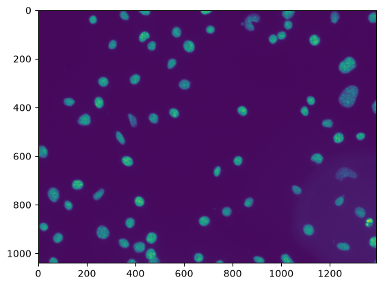
✍️ Exercise: View `filtered_image` with `matplotlib.pyplot`#

Remember to import what you need in setup!

plt.imshow(filtered_image)

<matplotlib.image.AxesImage at 0x7fac787c2270>

../../../_images/030a8e653c0981e9d6dde023d7695b739bef7135ddfb2317408247bce1f02f12.png

3. Thresholding#

Concept#

Thresholding is when we select a range of digital values, or intensity values, in the image. These selected values are how we define regions of the image we are interested in.

Defining a threshold#

We need to define a minimum intensity cutoff which separates the background (what we don’t care about) from the foreground (what we do care about). We can manually pick an intensity value, but picking an optimal value is tedious and may vary between images in a dataset. It is best practice to use established thresholding algorithms to automatically define an intensity cutoff value. skimage.filters contains many different types of thresholding algorithms, but from that we will be using the Otsu thresholding algorithm threshold_otsu.

Thresholding Algorithm	Description	How to import it	Documentation Link
Otsu thresholding	Returns threshold using Otsu’s method	`from skimage.filters import threshold_otsu`	threshold_otsu

Note: skimage.filters also has a try_all_threshold() function that takes an inputted image and returns a figure comparing the outputs of different thresholding methods. It can be a helpful tool to pick a good thresholding algorithm!

We can use threshold_otsu from skimage.filters as follows:

from skimage.filters import threshold_otsu # put in Setup
threshold = threshold_otsu(filtered_image)

Here, threshold_otsu() will use that inputted filtered_image to calculate an intensity cutoff value. It will return the cutoff value assigned to the variable threshold.

✍️ Exercise: Write code to calculate a threshold on `filtered_image` using Otsu’s method#

Remember - we need to import the threshold_otsu function from skimage.filters in Setup!

threshold = threshold_otsu(filtered_image)

Generating a binary mask#

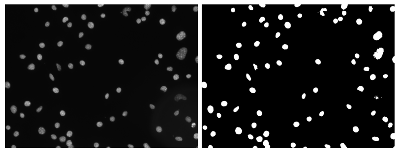
We now want to use this cutoff value to generate a binary mask, which is an image that has only 2 pixel values: one corresponding to the background and one corresponding to the foreground. By generating the binary mask, we will be able to evaluate whether this threshold is a sufficient cutoff value.

We can generate the binary mask by using the > comparison operator, since we want to accept values above a given threshold as foreground:

binary_mask = filtered_image > threshold

Python will interpret this line of code by going pixel by pixel through filtered_image and assigning True values where a pixel is greater than threshold and assigning False values where a pixel is equal or less than threshold. The output will be the binary mask image, filled with True and False.

✍️ Exercise: Write code to threshold `filtered_image` and generate a binary image assigned to the variable `binary_mask`. Print this image’s minimum and maximum values.#

binary_mask = filtered_image > threshold
print(np.max(binary_mask))  # binary_mask max value
print(np.min(binary_mask))  # binary_mask min value

True
False

Comparing the binary mask to the raw image#

We can use matplotlib.pyplot to view the raw_image and binary_mask side by side. We first need to import matplotlib.pyplot in Setup, which can be abbreviated as plt for simplicity.

Name	Description	How to import it	Documentation Link
`matplotlib.pyplot`	Creates interactive plots	`import matplotlib.pyplot as plt`	matplotlib.pyplot

Just as you learned in the last lesson, we can use plt.subplot() to plot multiple images. Plotting 2 images for side by side comparison is a very useful task, so let’s package this code into a function. You can get started with the template below:

import matplotlib.pyplot as plt # put in Setup

def double_image_plotter(img_1, img_2):
 
    # Create a figure
    # add code here!

    # Plot images
    # add code here!

    # Show the plot
    # add code here!

We can then call this double_image_plotter function whenever we want to plot 2 images side by side! We can do that by writing:

double_image_plotter(image_1, image_2)

✍️ Exercise: Write a function named `double_image_plotter` that uses `plt` to plot two images side by side.#

Remember to import matplotlib.pyplot as plt in Setup!

def double_image_plotter(img_1, img_2):
    """Function that plots 2 images side by side

    Parameters
    ----------
    img_1:
    left plotted image

    img_2:
    right plotted image

    Return
    ----------
    plot of the images

    """
    # Create a figure
    plt.figure(figsize=(8, 6), layout="constrained")

    # Plot images
    # img_1 in position 1
    plt.subplot(1, 2, 1)
    plt.imshow(img_1, cmap="gray", vmin=img_1.min(), vmax=img_1.max())
    plt.axis("off")  # Turn off axis

    #img_2 in position 2
    plt.subplot(1, 2, 2)
    plt.imshow(img_2, cmap="gray", vmin=img_2.min(), vmax=img_2.max())
    plt.axis("off")  # Turn off axis

    # Show the plot
    plt.show()

✍️ Exercise: View `dapi_image` and `binary_mask` side by side using the `double_image_plotter` function you just made.#

double_image_plotter(dapi_image, binary_mask)

../../../_images/115aa1f5bfb20384f62f11db18521a322bf8e49e78f8d8bd527b9d189ea59510.png

4. Mask Labeling#

Concept#

Now that we have a binary mask that has white, or value True, pixels that match the image foreground and black, or value False, pixels that match the image background, we can continue further to distinguish individual objects within this mask. Labeling a mask is when we identify individual objects within a binary mask and assign them a unique numerical identifier.

Labeling a binary mask#

From skimage.measure we can use label() to label a curated binary mask.

Function	Description	How to import it	Documentation Link
`label()`	Label connected regions of an image for Instance segmentation	`from skimage.measure import label`	skimage.measure.label

Here’s how we use label from skimage.measure to label a binary mask:

from skimage.measure import label # put in Setup
labeled_image = label(binary_mask)

Here, label() will take the inputted binary_mask and count each connected object in the image. It will then assign each object a whole number starting from 1. It will then return an image where each object’s pixels have the value of its object’s assigned number, which we assign to the variable labeled_image!

✍️ Exercise: Write code to label `binary_mask` and assign it to the variable `labeled_image`#

Remember - we need to import the label function from skimage.measure in Setup!

labeled_image = label(binary_mask)

Displaying a labeled mask on top of the image#

Let’s now summarize our final segmentation result in 1 image by viewing the labeled_image overlaid onto the original dapi_image. From skimage.color, we can use label2rgb to do this.

Function	Description	How to import it	Documentation Link
`label2rgb()`	Returns an RGB image where color-coded labels are painted over the image	`from skimage.color import label2rgb`	label2rgb

Here’s how we can use label2rgb from skimage.color to summarize our segmentation result:

from skimage.color import label2rgb # put in Setup
seg_summary = label2rgb(labeled_image, image = dapi_image)

Here, label2rgb() is filled with 2 arguments:

The labeled mask labeled_image
The original image we want the labeled_image overlaid onto, specified as image = dapi_image

The output will be an rgb image of the labeled mask overlaid onto the raw image, which is assigned to the variable seg_summary.

✍️ Exercise: Write code that creates an image of `labeled_image` overlaid onto `dapi_image` and assign it to the variable `seg_summary`#

Remember - we need to import the label2rgb function from skimage.color in Setup!

seg_summary = label2rgb(labeled_image, image=dapi_image)

✍️ Exercise: View `seg_summary` with `plt.imshow()`#

plt.imshow(seg_summary)
plt.axis("off")  # Turn off axis
plt.show()

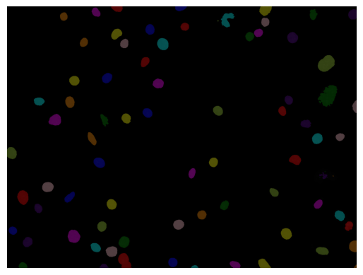
../../../_images/f780630f9678f7b5aeb5d0c232dc6d15d11f812db6d6905d2a45e919f74a9960.png

How does the segmentation result look? Are all labels corresponding to individual nuclei? If not, additional processing steps are needed to refine binary_mask.

5. Mask Refinement#

Concept#

Mask refinement is needed when a binary mask still does not accurately match the image foreground after filtering and thresholding. In the context of our nuclei example image, we need to apply additional processing steps to remove objects that are too small to be nuclei, fill any holes within nuclei, and separate touching nuclei.

Common mask refinement steps#

There are many different ways we can refine a binary mask. The table below summarizes the refinement steps we discussed in lecture:

Function Name	Description	How to import it	Documentation Link
`remove_small_objects()`	Removes objects smaller than the specified size from the foreground.	`from skimage.morphology import remove_small_objects`	skimage.morphology.remove_small_objects
`closing()`	Performs morphological closing, a mathematical operation that results in small hole removal	`from skimage.morphology import closing`	skimage.morphology.closing
`watershed()`	Performs the Watershed transform, a useful algorithm for separating touching round objects, such as nuclei. The output is a labeled image.	`from skimage.segmentation import watershed`	skimage.segmentation.watershed

Let’s now walk through steps to remove objects smaller than nuclei with remove_small_objects(), fill in any holes within nuclei with closing(), and then separate touching nuclei with watershed().

Removing objects smaller than nuclei#

In many cases, thresholding will be unsuccessful at rejecting image objects that are debris, as these tend to have high intensity values. However, we can use differences in object size to reject anything that is too small to be a nucleus.

From skimage.morphology we can use the remove_small_objects function to remove any connected objects of a specified min_size. Here is how we can do that:

from skimage.morphology import remove_small_objects # put in Setup
binary_mask_sized = remove_small_objects(binary_mask, min_size=10)

Here, remove_small_objects() will take the inputted binary_mask and set any connected object that is smaller than max_size=10 to have False values (in other words, be rejected as foreground). It will then return the updated binary mask, which we assigned to the variable binary_mask_sized.

✍️ Exercise: Write code to remove objects smaller than nuclei in `binary_mask` and assign it to the variable `binary_mask_sized`#

Remember, we need to import functions we want to use in Setup!

binary_mask_sized = remove_small_objects(binary_mask, min_size=50)

/tmp/ipykernel_3212/1787269595.py:1: FutureWarning: Parameter `min_size` is deprecated since version 0.26.0 and will be removed in 2.0.0 (or later). To avoid this warning, please use the parameter `max_size` instead. For more details, see the documentation of `remove_small_objects`. Note that the new threshold removes objects smaller than **or equal to** its value, while the previous parameter only removed smaller ones.
  binary_mask_sized = remove_small_objects(binary_mask, min_size=50)

NOTE: You may get a warning message about using min_size because in future offerings of the library it will be depreciated. Libraries change over time, so these warnings are meant to help keep you informed on how to properly use them. For now, we can continue as is because min_size is not depreciated yet!

✍️ Exercise: Use our `double_image_plotter` function to display `binary_mask` and `binary_mask_sized` side by side#

double_image_plotter(binary_mask, binary_mask_sized)

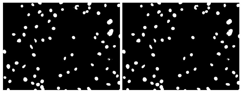
../../../_images/f63adfcf91848fb33b0dc463577768837eb2050779f39e2ed624c4cf54daa54d.png

Filling holes within nuclei#

While filtering helps reduce the effect of noise on thresholding, sometimes there will still be areas within an object that are below the minimum threshold value. These areas will show up as holes within a connected object. We can fill these holes by applying a morphological closing operation to the mask.

From skimage.morphology we can use the closing function to fill small holes within nuclei. Here is how we can do that:

from skimage.morphology import closing # put in Setup
from skimage.morphology import disk # put in Setup
binary_mask_filled = closing(binary_mask_sized, disk(1))

Here, closing() has two inputs:

The binary mask binary_mask_sized
A footprint disk(1), which is a disk shaped kernel of size 1

It uses these inputs to perform a morphological closing operation optimized for binary images. It will then return the updated binary mask, which we assign to the variable binary_mask_filled.

✍️ Exercise: Write code to fill holes within nuclei in `binary_mask_sized`, and assign the updated mask to the variable `binary_mask_filled`#

Remember, we need to import functions we want to use in Setup!

binary_mask_filled = closing(binary_mask_sized, disk(5))

✍️ Exercise: Use our `double_image_plotter` function to display `binary_mask_sized` and `binary_mask_filled`#

double_image_plotter(binary_mask_sized, binary_mask_filled)

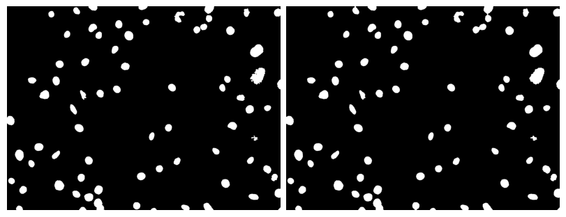
../../../_images/7982da0c2761a3a1462cf9a68549841e45d15ff33168b85c62a75d401ea0149d.png

Separating touching nuclei#

Let’s now apply the Watershed transform to our binary_mask to separate any touching nuclei. From skimage.segmentation, we can use watershed() to do this.

The watershed() function needs the following inputs:

The inverse of the distance transform of the binary mask
The seeds: labeled image of the peaks of the distance transform
The binary mask

We are going to need a few additional functions to provide the first two inputs to the watershed() function.

Function	Description	How to import it	Documentation Link
`distance_transform_edt()`	Calculates the distance transform of the input	`from scipy.ndimage import distance_transform_edt`	scipy.ndimage.distance_transform_edt
`peak_local_max`	Remove objects smaller than the specified size from the foreground.	`from skimage.feature import peak_local_max`	skimage.feature.peak_local_max

Computing the distance transform#

We can use the distance_transform_edt() function from scipy.ndimage to get the distance transform of our refined binary_mask binary_mask_filled:

from scipy.ndimage import distance_transform_edt # put in Setup
# compute the distance transform
distance_transform = distance_transform_edt(binary_mask_filled)

✍️ Exercise: Write code to calculate the distance transform of `binary_mask_filled` and assign it to the variable `distance_transform`#

Remember to import what you need in Setup!

# compute the distance transform
distance_transform = distance_transform_edt(binary_mask_filled)

Creating seeds for Watershed#

Once we have the distance transform of binary_mask_filled, we can use the peak_local_max() function from skimage.feature to get its local maxima. However, we want to make sure that we get only 1 local maximum per object. We therefore can apply a footprint input confine a region the peak_local_max function will look for local maxima. Doing so will constrain how many maxima the function returns. We can also specify a min_distance separating peaks, which will also help constrain the number of maxima to be 1 per nucleus.

Here’s how we would write the code:

from skimage.feature import peak_local_max # put in Setup
# find local maxima coordinates in the distance transform
local_maxima_coords = peak_local_max(distance_transform, footprint=np.ones((25, 25)), min_distance=10)

✍️ Exercise: Write code that finds the local maxima coordinates of `distance_transform`. Print the coordinates to see how they are organized.#

Remember to import what you need in Setup!

# find local maxima coordinates in the distance transform
local_maxima_coords = peak_local_max(
    distance_transform, footprint=np.ones((25, 25)), min_distance=10
)
print(local_maxima_coords)

[[ 364 1274]
 [ 231 1266]
 [ 221 1279]
 [ 915  266]
 [ 148  620]
 [ 581   14]
 [ 756   62]
 [ 451  193]
 [1005  463]
 [ 903 1112]
 [ 124 1137]
 [ 937  466]
 [ 975  416]
 [  31 1380]
 [ 525 1236]
 [ 717  163]
 [ 867  683]
 [ 621  368]
 [ 788  417]
 [ 294  268]
 [ 305  601]
 [ 608 1150]
 [ 379  250]
 [  91  569]
 [1018  660]
 [ 873  378]
 [ 283  399]
 [ 413  839]
 [ 423  560]
 [ 443  474]
 [ 936   83]
 [ 830 1324]
 [ 619  822]
 [ 829  775]
 [ 105  437]
 [ 119  966]
 [ 958  352]
 [  60 1029]
 [ 147  467]
 [ 377  126]
 [ 371 1122]
 [ 891   23]
 [ 216  551]
 [ 104 1002]
 [  79  708]
 [ 142  306]
 [ 466 1194]
 [ 415 1096]
 [ 972 1255]
 [  38  225]
 [ 791  866]
 [ 802  124]
 [ 519 1325]
 [ 870 1363]
 [ 741 1066]
 [  21  352]
 [ 786 1240]
 [  31 1220]
 [  64  868]
 [ 524  336]
 [ 663  736]
 [ 763  245]
 [ 451  389]
 [  37  873]
 [  35  891]
 [ 675 1264]]

Now that we have the local maxima, we need to organize them for the watershed() function as a labeled image. We can do that by creating a binary image that’s the same size as our binary mask. We will want all values in this new image to be False except where the local maxima are. Therefore, let’s use np.zeros_like() to create a binary image filled with False values that’s the same size as binary_mask:

#create image that's the same size and dtype as binary_mask_filled
local_maxima_image = np.zeros_like(binary_mask_filled, dtype=bool) 

✍️ Exercise: Write code that creates an image of `dtype=bool` that is the same size as `binary_mask`. Assign it to the variable `local_maxima_image`.#

# create image that's the same size and dtype as binary_mask_filled
local_maxima_image = np.zeros_like(binary_mask_filled, dtype=bool)

Now we need to add the local_maxima_coords to this new local_maxima_image. This is a tricky task, because local_maxima_coords organizes each (x,y) coordinate of where a local maximum is like this:

[[10, 20], # first peak at (row=10, col=20)
[30, 40], # second peak at (row=30, col=40)
[50, 60]] # third peak at (row=50, col=60)

We need a way to organize these coordinates so that we can insert all of the row and columns as separate arrays into local_maxima_coords. In other words, we need to organize the coordinates so they look like this:

[[10, 30, 50],  # all row indices
[20, 40, 60]]   # all column indices

We can start to do that by taking the transpose of local_maxima_coords. A transpose flips a matrix over its diagonal axis, effectively swapping rows and columns.

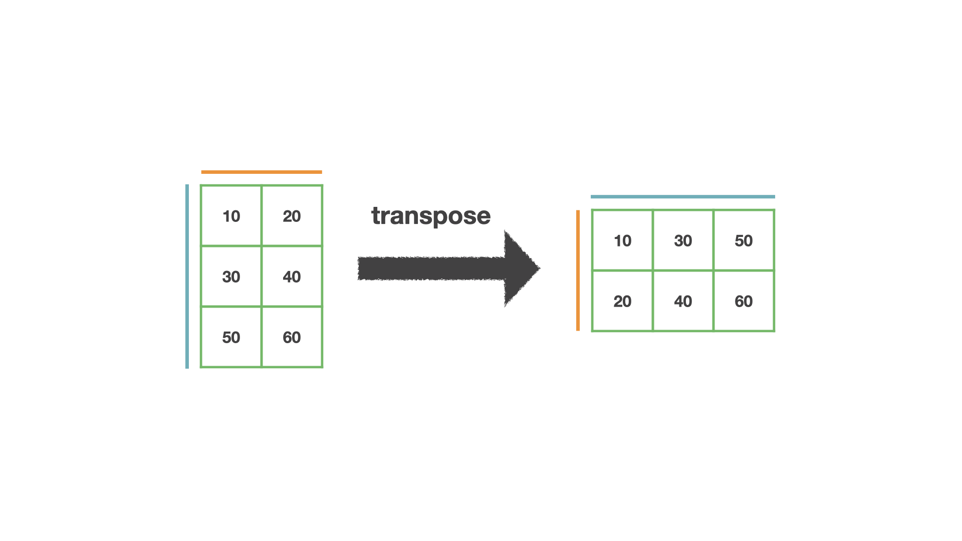
In Python, we take the transpose of an np.array by writing:

local_maxima_coords.T

Here, the “.T” indicates that we want the transpose of local_maxima_coords.

✍️ Exercise: Write code that takes the transpose of `local_maxima_coords`, then print the result.#

local_maxima_coords_transpose = local_maxima_coords.T
print(local_maxima_coords_transpose)

[[ 364  231  221  915  148  581  756  451 1005  903  124  937  975   31
717  867  621  788  294  305  608  379   91 1018  873  283  413
443  936  830  619  829  105  119  958   60  147  377  371  891
104   79  142  466  415  972   38  791  802  519  870  741   21
 31   64  524  663  763  451   37   35  675]
 [1274 1266 1279  266  620   14   62  193  463 1112 1137  466  416 1380
163  683  368  417  268  601 1150  250  569  660  378  399  839
474   83 1324  822  775  437  966  352 1029  467  126 1122   23
1002  708  306 1194 1096 1255  225  866  124 1325 1363 1066  352
1220  868  336  736  245  389  873  891 1264]]

We still have some work to do to get these coordinates into local_maxima_image. To pass the coordinates into local_maxima_image, we need to organize them as a tuple. We can do that with the tuple() function:

tuple(local_maxima_coords.T)

Now, the coordinates will be arranged as so:

array([10, 30, 50]),  # all row indices
array([20, 40, 60])   # all column indices

✍️ Exercise: Write code that converts the transpose of `local_maxima_coords` to a tuple. Print the result.#

local_maxima_coords_transpose = local_maxima_coords.T
local_maxima_coords_tuple = tuple(local_maxima_coords_transpose)
print(local_maxima_coords_tuple)

(array([ 364,  231,  221,  915,  148,  581,  756,  451, 1005,  903,  124,
        937,  975,   31,  525,  717,  867,  621,  788,  294,  305,  608,
        379,   91, 1018,  873,  283,  413,  423,  443,  936,  830,  619,
        829,  105,  119,  958,   60,  147,  377,  371,  891,  216,  104,
         79,  142,  466,  415,  972,   38,  791,  802,  519,  870,  741,
         21,  786,   31,   64,  524,  663,  763,  451,   37,   35,  675]), array([1274, 1266, 1279,  266,  620,   14,   62,  193,  463, 1112, 1137,
        466,  416, 1380, 1236,  163,  683,  368,  417,  268,  601, 1150,
        250,  569,  660,  378,  399,  839,  560,  474,   83, 1324,  822,
        775,  437,  966,  352, 1029,  467,  126, 1122,   23,  551, 1002,
        708,  306, 1194, 1096, 1255,  225,  866,  124, 1325, 1363, 1066,
        352, 1240, 1220,  868,  336,  736,  245,  389,  873,  891, 1264]))

This is exactly what we want them to look like to insert into local_maxima_image! Here’s how we can insert them:

local_maxima_image[tuple(local_maxima_coords.T)]

The last thing we need to do is make them all have value True, since local_maxima_image is a binary image. We can do that by writing:

# add local_maxima_coords to the created local_maxima_image, after organizing them
local_maxima_image[tuple(local_maxima_coords.T)] = True

✍️ Exercise: Write code that adds the `local_maxima_coords` to `local_maxima_image`.#

# organize the local maxima coordinates into a tuple of arrays for indexing
local_maxima_coords_transpose = local_maxima_coords.T
local_maxima_coords_tuple = tuple(local_maxima_coords_transpose)

# add the local_maxima_coords to the created local_maxima image
local_maxima_image[local_maxima_coords_tuple] = True

Finally, we can label local_maxima_image to create seeds for the Watershed function.

# label the local_maxima_image to create seeds for the watershed function
seeds = label(local_maxima_image)

Hooray! We have our seeds! Let’s now put all of what we just learned together about how we used distance_transform to create seeds.

✍️ Exercise: Put your code above together, starting with calculating the `distance_transform` to create seeds for the Watershed algorithm.#

# compute the distance transform
distance_transform = distance_transform_edt(binary_mask_filled)

# find local maxima coordinates in the distance transform
local_maxima_coords = peak_local_max(
    distance_transform, footprint=np.ones((25, 25)), min_distance=10
)

# create image that's the same size and dtype as binary_mask_filled
local_maxima_image = np.zeros_like(binary_mask_filled, dtype=bool)

# organize the local maxima coordinates into a tuple of arrays for indexing
local_maxima_coords_transpose = local_maxima_coords.T
local_maxima_coords_tuple = tuple(local_maxima_coords_transpose)

# add the local_maxima_coords to the created local_maxima image
local_maxima_image[local_maxima_coords_tuple] = True

# label the local_maxima image to create seeds for the watershed function
seeds = label(local_maxima_image)

Applying the Watershed Transform#

Now we have everything we need to input into the watershed() function:

The inverse of the distance transform of the binary mask: -distance_transform
The seeds: seeds
The binary mask: binary_mask_filled

We can now call the Watershed function as follows:

# apply the watershed algorithm to segment the image and get labels
from skimage.segmentation import watershed # put in Setup
labeled_ws_image = watershed(-distance_transform, seeds, mask=binary_mask_filled)

Here, watershed() will apply the Watershed Transform to the inputted binary_image_filled. It will return the transformed, labeled image. We assign it to the variable labeled_ws_image.

✍️ Exercise: Write code to apply a watershed transform to `binary_mask_filled` and assign it to the variable `labeled_ws_image`#

Remember to import what you need in Setup!

# apply the watershed algorithm to segment the image and get labels
labeled_ws_image = watershed(-distance_transform, seeds, mask=binary_mask_filled)

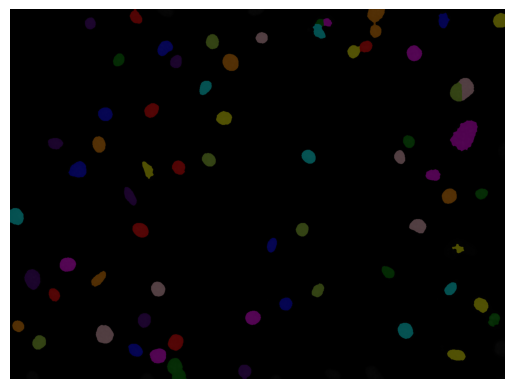
✍️ Exercise: Use `label2rgb()` to create an image of `labeled_ws_image` overlaid onto `dapi_image` and assign it to the variable `seg_summary_refined`#

seg_summary_refined = label2rgb(labeled_ws_image, image=dapi_image)

✍️ Exercise: Use `plt` to display `seg_summary_refined`#

plt.imshow(seg_summary_refined)
plt.axis("off")  # Turn off axis
plt.show()

../../../_images/e85c23d76f5a257265f2cc1dae523ed93c7843874727589dc60e066e9041babb.png

END OF FIRST LAB SECTION - STOP HERE FOR LAST LECTURE COMPONENT!#

6. Processing Many Images#

Concept#

Statistically relevant & reproducible measurements come from analyzing many fluorescence images. Therefore, we need to adapt our code to efficiently run on many images, not just 1 at a time! We can do so by implementing a for loop to our image path handling. We can also add the ability to save output files using tifffile.imwrite().

Consolidate code for image processing steps#

The first step to processing many images is to write code to process a single image, just as we have done above in the previous sections.

✍️ Exercise: Copy and paste all of the code we wrote in the above sections to load and segment our single nucleus image#

Remember, we want code that does the following steps:

Specify dependencies
Load the image
Filter the image with a Gaussian filter
Threshold to generate a binary mask
Refine the mask: Remove small objects
Refine the mask: Fill small holes
Refine the mask: Watershed

# specify dependencies
import matplotlib.pyplot as plt
import ndv
import numpy as np
import tifffile
from scipy.ndimage import distance_transform_edt
from skimage.color import label2rgb
from skimage.feature import peak_local_max
from skimage.filters import gaussian, threshold_otsu
from skimage.measure import label
from skimage.morphology import closing, disk, remove_small_objects
from skimage.segmentation import watershed

# load the image
image_path = r"../../../_static/images/classic_seg/DAPI_wf_0.tif"
raw_image = tifffile.imread(image_path)
dapi_image = raw_image[0]

# filter the image with gaussian filter
filtered_image = gaussian(dapi_image, sigma=1)

# threshold filtered_image to generate binary mask
binary_mask = filtered_image > threshold_otsu(filtered_image)

# Remove small objects
binary_mask_sized = remove_small_objects(binary_mask, min_size=50)

# Fill small holes by performing morphological closing
binary_mask_filled = closing(binary_mask_sized, disk(5))

# apply watershed to separate nuclei and label mask
# compute the distance transform
distance_transform = distance_transform_edt(binary_mask_filled)

# find local maxima coordinates in the distance transform
local_maxima_coords = peak_local_max(
    distance_transform, footprint=np.ones((25, 25)), min_distance=10
)

# create image that's the same size and dtype as binary_mask_filled
local_maxima_image = np.zeros_like(binary_mask_filled, dtype=bool)

# organize the local maxima coordinates into a tuple of arrays for indexing
local_maxima_coords_transpose = local_maxima_coords.T
local_maxima_coords_tuple = tuple(local_maxima_coords_transpose)

# add the local_maxima_coords to the created local_maxima image
local_maxima_image[local_maxima_coords_tuple] = True

# label the local_maxima image to create seeds for the watershed function
seeds = label(local_maxima_image)

# apply the watershed algorithm to segment the image and get labels
labeled_ws_image = watershed(-distance_transform, seeds, mask=binary_mask_filled)

/tmp/ipykernel_3212/2382838730.py:26: FutureWarning: Parameter `min_size` is deprecated since version 0.26.0 and will be removed in 2.0.0 (or later). To avoid this warning, please use the parameter `max_size` instead. For more details, see the documentation of `remove_small_objects`. Note that the new threshold removes objects smaller than **or equal to** its value, while the previous parameter only removed smaller ones.
  binary_mask_sized = remove_small_objects(binary_mask, min_size=50)

---------------------------------------------------------------------------
RuntimeError                              Traceback (most recent call last)
Cell In[30], line 29
     25 # Remove small objects
     26 binary_mask_sized = remove_small_objects(binary_mask, min_size=50)
     27 
     28 # Fill small holes by performing morphological closing
---> 29 binary_mask_filled = closing(binary_mask_sized, disk(5))
     30 
     31 # apply watershed to separate nuclei and label mask
     32 # compute the distance transform

File ~/work/bobiac-book/bobiac-book/.venv/lib/python3.12/site-packages/skimage/morphology/misc.py:47, in default_footprint.<locals>.func_out(image, footprint, *args, **kwargs)
     45 if footprint is None:
     46     footprint = ndi.generate_binary_structure(image.ndim, 1)
---> 47 return func(image, footprint=footprint, *args, **kwargs)

File ~/work/bobiac-book/bobiac-book/.venv/lib/python3.12/site-packages/skimage/morphology/gray.py:436, in closing(image, footprint, out, mode, cval)
    366 """Return grayscale morphological closing of an image.
    367 
    368 The morphological closing of an image is defined as a dilation followed by
   (...)    433 
    434 """
    435 footprint = pad_footprint(footprint, pad_end=False)
--> 436 dilated = dilation(image, footprint, mode=mode, cval=cval)
    437 out = erosion(dilated, mirror_footprint(footprint), out=out, mode=mode, cval=cval)
    438 return out

File ~/work/bobiac-book/bobiac-book/.venv/lib/python3.12/site-packages/skimage/morphology/misc.py:47, in default_footprint.<locals>.func_out(image, footprint, *args, **kwargs)
     45 if footprint is None:
     46     footprint = ndi.generate_binary_structure(image.ndim, 1)
---> 47 return func(image, footprint=footprint, *args, **kwargs)

File ~/work/bobiac-book/bobiac-book/.venv/lib/python3.12/site-packages/skimage/morphology/gray.py:276, in dilation(image, footprint, out, mode, cval)
    273 if not _footprint_is_sequence(footprint):
    274     footprint = [(footprint, 1)]
--> 276 out = _iterate_gray_func(
    277     gray_func=ndi.grey_dilation,
    278     image=image,
    279     footprints=footprint,
    280     out=out,
    281     mode=mode,
    282     cval=cval,
    283 )
    284 return out

File ~/work/bobiac-book/bobiac-book/.venv/lib/python3.12/site-packages/skimage/morphology/gray.py:22, in _iterate_gray_func(gray_func, image, footprints, out, mode, cval)
     16 """Helper to call `gray_func` for each footprint in a sequence.
     17 
     18 `gray_func` is a morphology function that accepts `footprint`, `output`,
     19 `mode` and `cval` keyword arguments (e.g. `scipy.ndimage.grey_erosion`).
     20 """
     21 fp, num_iter = footprints[0]
---> 22 gray_func(image, footprint=fp, output=out, mode=mode, cval=cval)
     23 for _ in range(1, num_iter):
     24     gray_func(out.copy(), footprint=fp, output=out, mode=mode, cval=cval)

File ~/work/bobiac-book/bobiac-book/.venv/lib/python3.12/site-packages/scipy/ndimage/_morphology.py:1444, in grey_dilation(input, size, footprint, structure, output, mode, cval, origin, axes)
   1441     if not sz & 1:
   1442         origin[ii] -= 1
-> 1444 return _filters._min_or_max_filter(input, size, footprint, structure,
   1445                                    output, mode, cval, origin, 0,
   1446                                    axes=axes)

File ~/work/bobiac-book/bobiac-book/.venv/lib/python3.12/site-packages/scipy/ndimage/_filters.py:1799, in _min_or_max_filter(input, size, footprint, structure, output, mode, cval, origin, minimum, axes)
   1797 fshape = [ii for ii in footprint.shape if ii > 0]
   1798 if len(fshape) != input.ndim:
-> 1799     raise RuntimeError(f"footprint.ndim ({footprint.ndim}) must match "
   1800                        f"len(axes) ({len(axes)})")
   1801 for origin, lenf in zip(origins, fshape):
   1802     if (lenf // 2 + origin < 0) or (lenf // 2 + origin >= lenf):

RuntimeError: footprint.ndim (2) must match len(axes) (1)

Using a `for` loop to loop through image paths#

Now that we have the code in one place, we need to adapt it to be able to process more than one image. We can do that by looping through image file paths. From pathlib, we can use Path in conjunction with a for loop to iterate through many image file paths in a specified folder directory. Here’s how we would write the code to do that:

from pathlib import Path
folder_dir = Path("/Users/edelase/bobiac/") # update with your folder directory
for image_path in folder_dir.iterdir():
    # do things

Providing the function Path with a folder directory points Python to the folder we want to access files from. We assign it to the variable folder_dir to make it easy to work with. Writing folder_dir.iterdir() points to this folder we want to work in, and hands us all file paths within the folder. Since we want to loop through each file path in the folder, we set up our for loop to take each image_path within what folder_dir.iterdir() provides from the folder. We can then do whatever tasks we would like for each image_path.

✍️ Exercise: Write a for loop that prints all image file paths in a folder using `Path` and `iterdir()`#

from pathlib import Path

folder_dir = Path("../../../_static/images/classic_seg/")
for image_path in folder_dir.iterdir():
    print(image_path)

Using `glob` to loop through only tif image paths#

What if we have more than just tif images in our folder? Instead of using iterdir(), we can selectively loop through files ending with “.tif” using glob. Here’s how we would write the code to do that:

from pathlib import Path
folder_dir = Path("/Users/edelase/bobiac/")
for image_path in folder_dir.glob("*.tif"): # only loop through files ending in .tif
    # do things

Here, we are still using Path to point Python to the folder we want to access files from. However, instead of using iterdir() to hand us all file paths within the folder, we are using glob to only hand us file paths in the folder ending with “.tif”. We are then looking through each of these file paths.

✍️ Exercise: Write a for loop that prints all tif image file paths in a folder using `Path` and `glob`#

from pathlib import Path

folder_dir = Path("../../../_static/images/classic_seg/")
for image_path in folder_dir.glob("*.tif"):  # only loop through files ending in .tif
    print(image_path)

Using a `for` loop to process many images#

Now that we have learned how to loop through image paths efficiently, we can now apply this concept to increase the throughput of our classic segmentation processing code. We can do that by putting each processing step, starting with reading the image, within the for loop.

from pathlib import Path
folder_dir = Path("/Users/edelase/bobiac/")
for image_path in folder_dir.glob("*.tif"): # only loop through files ending in .tif
    # load the image
    raw_image = tifffile.imread(image_path)
    ...
    break # Use for troubleshooting! Only do first loop until confident you're ready to loop through all files

Here, Python will loop through each image_path ending with “.tif” in folder_dir and conduct the indented lines of code. Until we’re ready to loop through all images and complete processing steps, we can use break as a last indented step in our for loop to only complete 1 loop.

✍️ Exercise: Improve your classic segmentation code above by adding a for loop to process many images#

from pathlib import Path

import numpy as np
import tifffile
from scipy.ndimage import distance_transform_edt
from skimage.feature import peak_local_max
from skimage.filters import gaussian, threshold_otsu
from skimage.measure import label
from skimage.morphology import closing, disk, remove_small_objects
from skimage.segmentation import watershed

folder_dir = Path("../../../_static/images/classic_seg/")

for image_path in folder_dir.glob("*.tif"):  # only loop through files ending in .tif
    # load the image
    raw_image = tifffile.imread(image_path)
    dapi_image = raw_image[0]

    # filter the image with gaussian filter
    filtered_image = gaussian(dapi_image, sigma=1)

    # threshold filtered_image to generate binary mask
    binary_mask = filtered_image > threshold_otsu(filtered_image)

    # Remove small objects
    binary_mask_sized = remove_small_objects(binary_mask, min_size=50)

    # Fill small holes by performing morphological closing
    binary_mask_filled = closing(binary_mask_sized, disk(5))

    # apply watershed to separate nuclei and label mask
    # compute the distance transform
    distance_transform = distance_transform_edt(binary_mask_filled)

    # find local maxima coordinates in the distance transform
    local_maxima_coords = peak_local_max(
        distance_transform, footprint=np.ones((25, 25)), min_distance=10
    )

    # create image that's the same size and dtype as binary_mask_filled
    local_maxima_image = np.zeros_like(binary_mask_filled, dtype=bool)

    # organize the local maxima coordinates into a tuple of arrays for indexing
    local_maxima_coords_transpose = local_maxima_coords.T
    local_maxima_coords_tuple = tuple(local_maxima_coords_transpose)

    # add the local_maxima_coords to the created local_maxima image
    local_maxima_image[local_maxima_coords_tuple] = True

    # label the local_maxima image to create seeds for the watershed function
    seeds = label(local_maxima_image)

    # apply the watershed algorithm to segment the image and get labels
    labeled_ws_image = watershed(-distance_transform, seeds, mask=binary_mask_filled)

    break

Saving Output Files#

Now that we have our for loop set up, we can modify our code to save the labeled_ws_image as an outputted tif file. We can do this using tifffile.imwrite(). Here’s how we can write the code:

output_dir = Path("/Users/edelase/bobiac/results")
tifffile.imwrite(output_dir/"output_image.tif", data=labeled_ws_image.astype("uint32"))

Here, tifffile.imwrite is provided with 3 inputs:

output_dir/"output_image.tif" is the file path the image will be saved to, which ends with a specified file name
data=labeled_ws_image.astype("uint32") is specifying the image to save and specifying that it be saved as “uint32”, or 32 bit

tifffile.imread() will use these inputs to output a file saved to the output_dir folder.

NOTE: The dtype of a labeled image is important because it determines the maximum number of labels stored in the image. Since each object in a labeled image is assigned a unique integer label, the dtype determines the range of integers that can be used for this labeling (e.g. uint8 -> max 255 objects). By default, labels generated by the skimage.measure.label() function are of type uint32.

When we provide tifffile.imwrite() with an output file path, we run into a problem. We can’t just directly write, or hard code, a file name for the image we are trying to save because it will be different for each iteration of our for loop. Therefore, we need a way to automatically generate a file name for each loop. We can do this by accessing the stem of a given image_path, which would give us the starting file name without the .tif at the end:

image_path.stem # returns file name, without .tif at the end, from image_path

Let’s see this in action!

✍️ Exercise: Print the file name of each tif image in your folder using `stem`#

folder_dir = Path("../../../_static/images/classic_seg/")
for image_path in folder_dir.glob("*.tif"):  # only loop through files ending in .tif
    print(image_path.stem)  # file name, without .tif at the end

However, we want to add a “.tif” at the end, as well as an additional label to the file name to distinguish it from the original raw_image. We can use an f-string to add a “_labeled.tif” at the end of the file name:

f"{image_path.stem}_labeled.tif"

Together, this will give us the full file name to save the image. To make it a full file path, we can combine it with our output_dir:

output_filepath = output_dir/f"{image_path.stem}_labeled.tif"

Now, let’s apply these modifications to our image processing code:

input_dir = Path("/Users/edelase/bobiac/")
output_dir = Path("/Users/edelase/bobiac/results")
for image_path in input_dir.glob("*.tif"): # only loop through files ending in .tif
    # do processing steps

    # save file
    output_filepath = output_dir/f"{image_path.stem}_labeled.tif"
    tifffile.imwrite(output_filepath, data = labeled_ws_image.astype("uint32"))

Now, let’s apply these concepts to our segmentation code so that we can save each final labeled image as an outputted tif file.

✍️ Exercise: Modify your classic segmentation code that processes many images to save each `labeled_ws_image`#

from pathlib import Path

import numpy as np
import tifffile
from scipy.ndimage import distance_transform_edt
from skimage.feature import peak_local_max
from skimage.filters import gaussian, threshold_otsu
from skimage.measure import label
from skimage.morphology import closing, disk, remove_small_objects
from skimage.segmentation import watershed

input_dir = Path("../../../_static/images/classic_seg/")
output_dir = Path("../../../_static/images/classic_seg/")

for image_path in input_dir.glob("*.tif"):  # only loop through files ending in .tif
    # load the image
    raw_image = tifffile.imread(image_path)
    dapi_image = raw_image[0]

    # filter the image with gaussian filter
    filtered_image = gaussian(dapi_image, sigma=1)

    # threshold filtered_image to generate binary mask
    binary_mask = filtered_image > threshold_otsu(filtered_image)

    # Remove small objects
    binary_mask_sized = remove_small_objects(binary_mask, min_size=50)

    # Fill small holes by performing morphological closing
    binary_mask_filled = closing(binary_mask_sized, disk(5))

    # apply watershed to separate nuclei and label mask
    # compute the distance transform
    distance_transform = distance_transform_edt(binary_mask_filled)

    # find local maxima coordinates in the distance transform
    local_maxima_coords = peak_local_max(
        distance_transform, footprint=np.ones((25, 25)), min_distance=10
    )

    # create image that's the same size and dtype as binary_mask_filled
    local_maxima_image = np.zeros_like(binary_mask_filled, dtype=bool)

    # organize the local maxima coordinates into a tuple of arrays for indexing
    local_maxima_coords_transpose = local_maxima_coords.T
    local_maxima_coords_tuple = tuple(local_maxima_coords_transpose)

    # add the local_maxima_coords to the created local_maxima image
    local_maxima_image[local_maxima_coords_tuple] = True

    # label the local_maxima image to create seeds for the watershed function
    seeds = label(local_maxima_image)

    # apply the watershed algorithm to segment the image and get labels
    labeled_ws_image = watershed(-distance_transform, seeds, mask=binary_mask_filled)

    # save labeled_ws_image
    output_filename = output_dir / f"{image_path.stem}_labeled.tif"
    tifffile.imwrite(output_filename, data=labeled_ws_image.astype("uint32"))

    break

When you are happy with the code, simply remove the break statement to run the code on all images in the folder.

Next Steps#

Congratulations for making it to the end of this lesson! You have now started learning how to segment and process many images in Python! However, just as with syntax, there is always more to learn when it comes to mastering a programming language and mindset. Below is a problem set we recommend to review concepts and build upon your new-found knowledge.

1. BoBiAC Exercises: Classic Segmentation

Classical Segmentation

Contents

Classical Segmentation#

Overview#

0. Setup#

Concept#

✍️ Exercise: Specify dependencies and run the code block for each section#

1. Loading an Image#

Concept#

✍️ Exercise: Use tifffile to read the image and assign it to the variable raw_image. Then, print its shape and dtype.#

✍️ Exercise: Use ndv to view the image raw_image.#

✍️ Exercise: Use numpy array indexing to get the DAPI image. Assign it to the variable dapi_image.#

2. Filtering#

Concept#

Applying a filter to an image#

✍️ Exercise: Write code to apply a Gaussian blur filter to dapi_image and assign it to the variable filtered_image#

✍️ Exercise: View filtered_image with matplotlib.pyplot#

3. Thresholding#

Concept#

Defining a threshold#

✍️ Exercise: Write code to calculate a threshold on filtered_image using Otsu’s method#

Generating a binary mask#

✍️ Exercise: Write code to threshold filtered_image and generate a binary image assigned to the variable binary_mask. Print this image’s minimum and maximum values.#

Comparing the binary mask to the raw image#

✍️ Exercise: Write a function named double_image_plotter that uses plt to plot two images side by side.#

✍️ Exercise: View dapi_image and binary_mask side by side using the double_image_plotter function you just made.#

4. Mask Labeling#

Concept#

Labeling a binary mask#

✍️ Exercise: Write code to label binary_mask and assign it to the variable labeled_image#

Displaying a labeled mask on top of the image#

✍️ Exercise: Write code that creates an image of labeled_image overlaid onto dapi_image and assign it to the variable seg_summary#

✍️ Exercise: View seg_summary with plt.imshow()#

5. Mask Refinement#

Concept#

Common mask refinement steps#

Removing objects smaller than nuclei#

✍️ Exercise: Write code to remove objects smaller than nuclei in binary_mask and assign it to the variable binary_mask_sized#

✍️ Exercise: Use our double_image_plotter function to display binary_mask and binary_mask_sized side by side#

Filling holes within nuclei#

✍️ Exercise: Write code to fill holes within nuclei in binary_mask_sized, and assign the updated mask to the variable binary_mask_filled#

✍️ Exercise: Use our double_image_plotter function to display binary_mask_sized and binary_mask_filled#

Separating touching nuclei#

Computing the distance transform#

✍️ Exercise: Write code to calculate the distance transform of binary_mask_filled and assign it to the variable distance_transform#

Creating seeds for Watershed#

✍️ Exercise: Write code that finds the local maxima coordinates of distance_transform. Print the coordinates to see how they are organized.#

✍️ Exercise: Write code that creates an image of dtype=bool that is the same size as binary_mask. Assign it to the variable local_maxima_image.#

✍️ Exercise: Write code that takes the transpose of local_maxima_coords, then print the result.#

✍️ Exercise: Write code that converts the transpose of local_maxima_coords to a tuple. Print the result.#

✍️ Exercise: Write code that adds the local_maxima_coords to local_maxima_image.#

✍️ Exercise: Put your code above together, starting with calculating the distance_transform to create seeds for the Watershed algorithm.#

Applying the Watershed Transform#

✍️ Exercise: Write code to apply a watershed transform to binary_mask_filled and assign it to the variable labeled_ws_image#

✍️ Exercise: Use label2rgb() to create an image of labeled_ws_image overlaid onto dapi_image and assign it to the variable seg_summary_refined#

✍️ Exercise: Use plt to display seg_summary_refined#

END OF FIRST LAB SECTION - STOP HERE FOR LAST LECTURE COMPONENT!#

6. Processing Many Images#

Concept#

Consolidate code for image processing steps#

✍️ Exercise: Copy and paste all of the code we wrote in the above sections to load and segment our single nucleus image#

Using a for loop to loop through image paths#

✍️ Exercise: Write a for loop that prints all image file paths in a folder using Path and iterdir()#

Using glob to loop through only tif image paths#

✍️ Exercise: Write a for loop that prints all tif image file paths in a folder using Path and glob#

Using a for loop to process many images#

✍️ Exercise: Improve your classic segmentation code above by adding a for loop to process many images#

Saving Output Files#

✍️ Exercise: Print the file name of each tif image in your folder using stem#

✍️ Exercise: Modify your classic segmentation code that processes many images to save each labeled_ws_image#

Next Steps#

✍️ Exercise: Use `tifffile` to read the image and assign it to the variable `raw_image`. Then, print its shape and dtype.#

✍️ Exercise: Use `ndv` to view the image `raw_image`.#

✍️ Exercise: Use `numpy` array indexing to get the DAPI image. Assign it to the variable `dapi_image`.#

✍️ Exercise: Write code to apply a Gaussian blur filter to `dapi_image` and assign it to the variable `filtered_image`#

✍️ Exercise: View `filtered_image` with `matplotlib.pyplot`#

✍️ Exercise: Write code to calculate a threshold on `filtered_image` using Otsu’s method#

✍️ Exercise: Write code to threshold `filtered_image` and generate a binary image assigned to the variable `binary_mask`. Print this image’s minimum and maximum values.#

✍️ Exercise: Write a function named `double_image_plotter` that uses `plt` to plot two images side by side.#

✍️ Exercise: View `dapi_image` and `binary_mask` side by side using the `double_image_plotter` function you just made.#

✍️ Exercise: Write code to label `binary_mask` and assign it to the variable `labeled_image`#

✍️ Exercise: Write code that creates an image of `labeled_image` overlaid onto `dapi_image` and assign it to the variable `seg_summary`#

✍️ Exercise: View `seg_summary` with `plt.imshow()`#

✍️ Exercise: Write code to remove objects smaller than nuclei in `binary_mask` and assign it to the variable `binary_mask_sized`#

✍️ Exercise: Use our `double_image_plotter` function to display `binary_mask` and `binary_mask_sized` side by side#

✍️ Exercise: Write code to fill holes within nuclei in `binary_mask_sized`, and assign the updated mask to the variable `binary_mask_filled`#

✍️ Exercise: Use our `double_image_plotter` function to display `binary_mask_sized` and `binary_mask_filled`#

✍️ Exercise: Write code to calculate the distance transform of `binary_mask_filled` and assign it to the variable `distance_transform`#

✍️ Exercise: Write code that finds the local maxima coordinates of `distance_transform`. Print the coordinates to see how they are organized.#

✍️ Exercise: Write code that creates an image of `dtype=bool` that is the same size as `binary_mask`. Assign it to the variable `local_maxima_image`.#

✍️ Exercise: Write code that takes the transpose of `local_maxima_coords`, then print the result.#

✍️ Exercise: Write code that converts the transpose of `local_maxima_coords` to a tuple. Print the result.#

✍️ Exercise: Write code that adds the `local_maxima_coords` to `local_maxima_image`.#

✍️ Exercise: Put your code above together, starting with calculating the `distance_transform` to create seeds for the Watershed algorithm.#

✍️ Exercise: Write code to apply a watershed transform to `binary_mask_filled` and assign it to the variable `labeled_ws_image`#

✍️ Exercise: Use `label2rgb()` to create an image of `labeled_ws_image` overlaid onto `dapi_image` and assign it to the variable `seg_summary_refined`#

✍️ Exercise: Use `plt` to display `seg_summary_refined`#

Using a `for` loop to loop through image paths#

✍️ Exercise: Write a for loop that prints all image file paths in a folder using `Path` and `iterdir()`#

Using `glob` to loop through only tif image paths#

✍️ Exercise: Write a for loop that prints all tif image file paths in a folder using `Path` and `glob`#

Using a `for` loop to process many images#

✍️ Exercise: Print the file name of each tif image in your folder using `stem`#

✍️ Exercise: Modify your classic segmentation code that processes many images to save each `labeled_ws_image`#